Week 5 - Rayleigh Taylor Instability

AIM:

Rayleigh Taylor Instability

Objectives:

1. What are some practical CFD models that have been based on the mathematical analysis of Rayleigh Taylor waves? In your own words, explain how these mathematical models have been adapted for CFD calculations.
2. Perform the Rayleigh Taylor instability simulation for 2 different mesh sizes with the base mesh being 0.5 mm. Compare the results by showing the animations( Attach them from your google drive). Observe the differences in the animation and explain the effect of mesh size on simulation. Also, explain why a steady-state approach might not be suitable for these types of simulation.[ Choose Air and Water for this simulation]
3. Run one more simulation with water and user-defined material(density = 400 kg/m³, viscosity = 0.001 kg/m-s) for refined mesh.
4. Define the Atwood Number. Find out the Atwood number for both the cases and explain how the variation in Atwood number in the above two cases affects the behavior of the instability.

Thory:

Rayleigh taylor instability:

Rayleigh-Taylor instability occurs in a system with two fluids in the presence of the gravity field or acceleration field. The fluid with higher density is located above the fluid with smaller density. Due to the gravity in the system fluid with higher density moves below the fluid with lower density. Interphase between the phases develops into structure similar to cosine wave and later to mushroom-like structures. The system of two immiscible fluids is analyzed.Examples include the behavior of water suspended above oil in the gravity of earth and atmospheric nuclear explosions.

1.What are some practical CFD models that have been based on the mathematical analysis of Rayleigh Taylor waves? In your own words, explain how these mathematical models have been adapted for CFD calculations.

some practical CFD models are

volume of fluid model-

volume of fluid model also called single fluid model. Volume of fluid (VOF) method (Hirt and Nichols 1981) introduces a continuity equation for the volume of fluid. In later implementations the numerical diffusion of the interface is eliminated with the reconstruction of the interface from the volume fraction in computational cells with the geometrical elements. This method is based on the idea of a so-called fraction function C. It is a scalar function, defined as the integral of a fluid's charecterstic function in the control volume, namely the volume of a computational grid cell. The volume fraction of each fluid is tracked through every cell in the computational grid, while all fluids share a single set of momentum equations. When a cell is empty with no traced fluid inside, the value of C is zero; when the cell is full, C = 1 and when there is a fluid interface in the cell, 0<C<1. C is a discontinuous function, its value jumps from 0 to 1 when the argument moves into interior of traced phase. based upon the value of C, we can see how the fluid and air ocuupied in a cell. Two-dimensional continuity equation, momentum equation, and continuity equation for volume fraction form a system of Navier-Stokes equations were used in this model.

two fluid model-

when the flow beside free surface also involves dispersed phase with the structures smaller then the grid size they are not appropriate. For dispersed flows two-fluid model is used, but the same model can also be used for simulations of flows with free surface. In future two-fluid model could be used for simulation of flows with free surface and dispersed phase. Two-fluid model consists of system of Navier-Stokes equations
for each phase.

concervative level set model-

The numerical diffusion of the interface is a big disadvantage of two-fluid model used for simulation of free surface flows. better reduction of numerical diffusion of the interface can be achieved with interface sharpening which is called conservative level set method.

2.Perform the Rayleigh Taylor instability simulation for 2 different mesh sizes with the base mesh being 0.5 mm. Compare the results by showing the animations( Attach them from your google drive). Observe the differences in the animation and explain the effect of mesh size on simulation. Also, explain why a steady-state approach might not be suitable for these types of simulation.[ Choose Air and Water for this simulation]

geometry:

here we are going to simulate for a 2d flow. so first we have to create a plane with equal sides, name the geometry as 'air'. after that we are going to create a plane on the top of the air geoemtry and we have to name it as 'water'. i have taken xz plane here. in the figure we named the top plane as air and bottem plane as water, as the direction of z is along the downword direction. fluent has a special feature that when we open geometry the direction of z axis gets along upword direction. so we can finally get that top plane as water and the bottem plane as air.

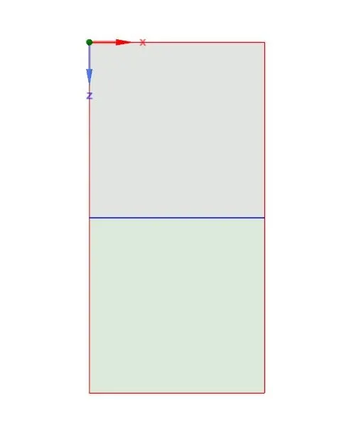
i have named the top plane as water and the bottem plane as air beacause higher density fluids must be on the top of the lower density fluid.

mesh:

with element size is 0.5mm-

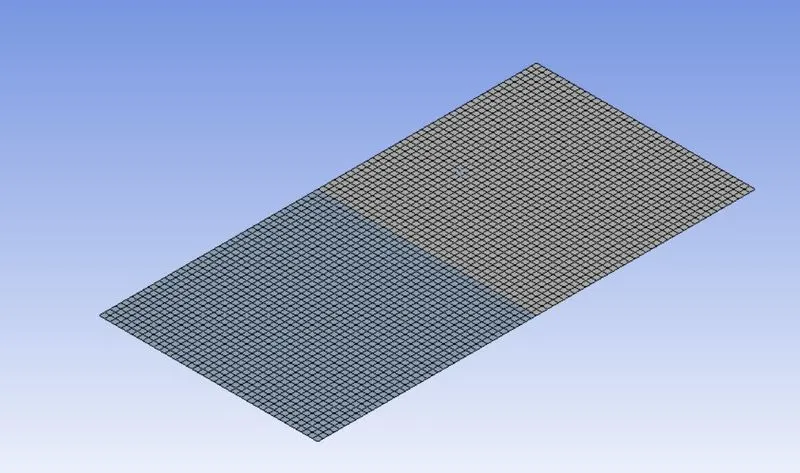
total number of cells obtained are 3200

setup:

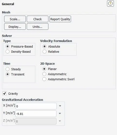
as the plane as a 2d plane. the fluent has a feature that in whatever plane we have craeted a 2d model, the fluent tak the plane as xy plane. here i have taken gravitational accaleration because the high density fluid moves downword due to gravity. i have taken transient state approach because we are going to see how the interphase gets collapsed with time. we are focussing at interphase becaues there will be numerical diffusion will occur which is not good to study the instability of the fluid.

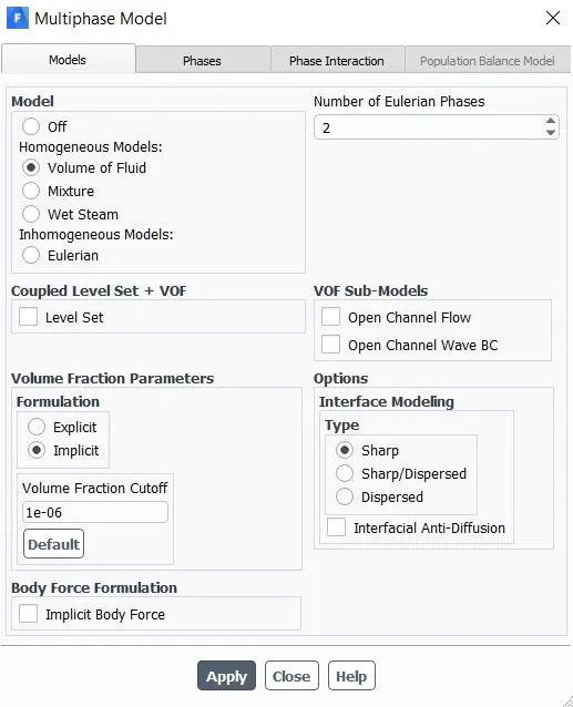
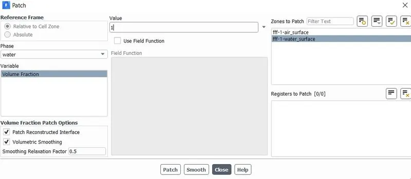
as there two phases gets involved so we have to enable multi phase model. in multi phase model i have taken volume of fluid method. here the fluid flow i taken as laminar flow. i have taken the time step size as 0.005 and the number of time steps are 1500. after initialization open patch and take the volume fraction of water as 1 and and click on patch and again take air fraction as 0 and click on patch.

solution:

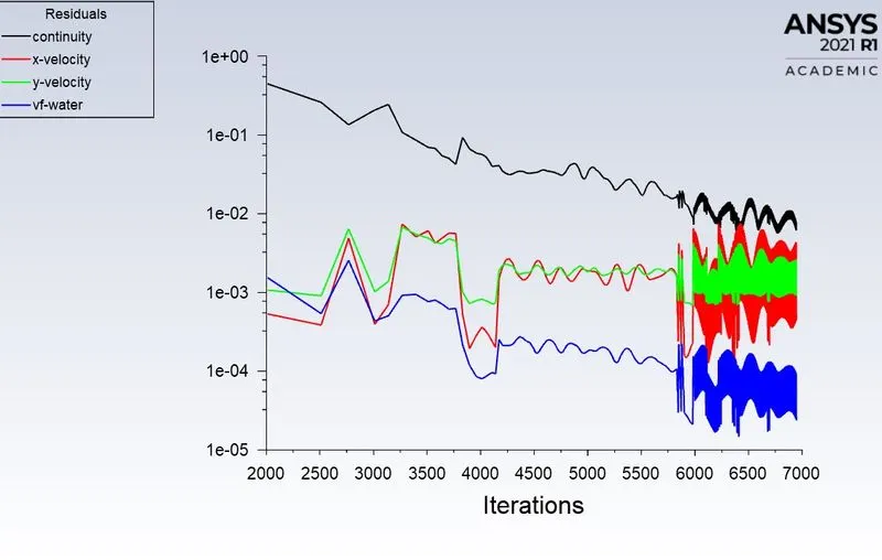
after calculation for 1500 time steps the final obtained plots are

residuals plot-

contour of volume fraction(water)-

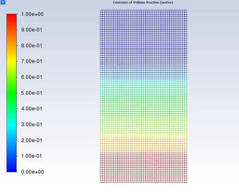
animation link for the above contour-

https://drive.google.com/file/d/1mqhKJRiYDZ2qxhhACr0nVmP4L7llSF7V/view?usp=sharing

refined mesh:

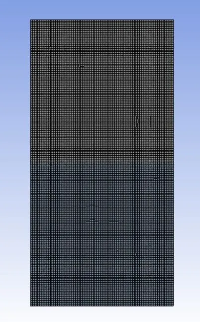
here i have taken the element size as 0.25mm and the total number of elements created are 12800.

solution:

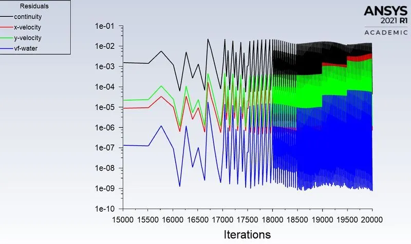
residuals plot-

contour of volume fraction(water)-

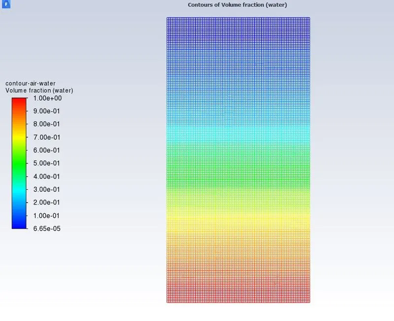
by reducing the size of the cell we can clearly isualize that the fluid flow gets unstabled at each cell. the numerical diffusion at interphase also gets reduced due to decrease of size of the cell and also the fluid reached to steady state position with less number of times stpes compared to base line mesh.

animation link for the above refined contour-

https://drive.google.com/file/d/14SrzM-q_nsYPAEWELzszix7ARqyOXCpd/view?usp=sharing

3.Run one more simulation with water and user-defined material(density = 400 kg/m³, viscosity = 0.001 kg/m-s) for refined mesh-

solution:

by taking user material of density = 400 kg/m³and viscosity = 0.001 kg/m-s

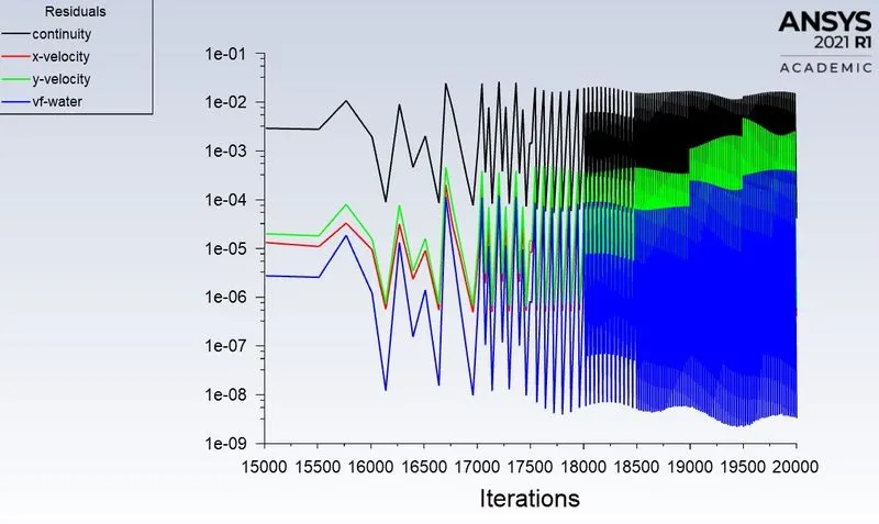
the residuals plot-

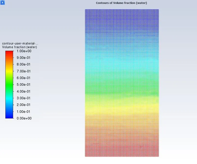
contour of volume fraction(water)-

animation link for the above refined contour-

https://drive.google.com/file/d/1bEV89UQ02uR_fOegA0n12e2BZJ4ZPrCU/view?usp=sharing

4. Atwood number:

The Atwood number (A) is a dimensionless number in fluid dynamics used in the study of hydraulic instabilities in density stratified flows(stratified flouid is defined as the fluid with density variations in the vertical direction). Atwood number is an important parameter in the study of Rayleigh–Taylor instability. For Atwood number close to 0, RT instability flows take the form of symmetric “fingers” of fluid; for Atwood number close to 1, the much lighter fluid “below” the heavier fluid takes the form of larger bubble-like plumes It is a dimensionless density ratio defined as

`A = (rho1-rho2)/(rho1+rho2`

where

`rho1`= density of heavier fluid

`rho2` = density of lighter fluid

for air-

density = 1.225kg/m³

for water-

density = 1000kg/m³

atwood number(A) = (1000-1.225)/(1000+1.225) = 0.9975

for user material-

density = 400kg/m³

^{for water-}

^{density = 1000kg/m3}

^{atwood number(A) = (1000-400)/(1000+400) = 0.428}

the atwood number is close to 1 for the above above simulation with air and water as fluids. while watching the animation video we can clearly see that there are large air bubble like plumes got developed during the water flows downwords due to gravity. so we can say the here atwood is valid. the atwood number for user material and water is in between 0 to 1, while seeing the animation video we can see that the small fingers and small plumes got developed.