Week 3 - External flow simulation over an Ahmed body.

AIM:

External flow simulation over an Ahmed body

Theory:

Ahmed body and its importance:

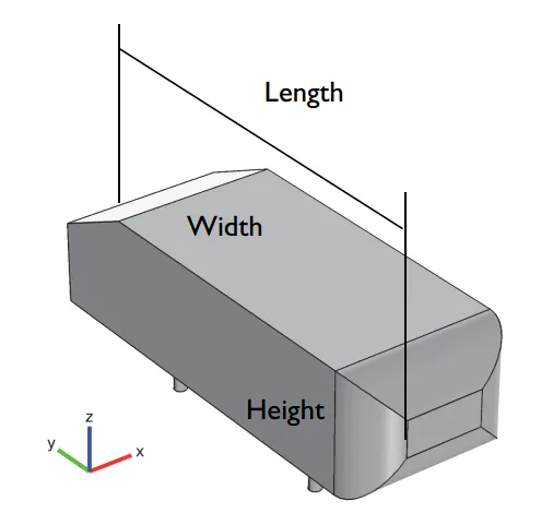
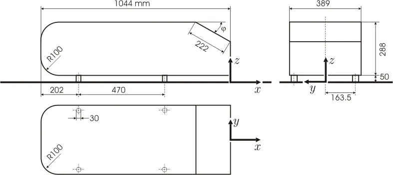
As the burning of fossil fuels becomes a more pressing issue, manufacturers are introducing more fuel efficient cars to the market. One main contributor to fuel burn is the car’s aerodynamic drag. Complexly shaped, cars are very challenging to model and it’s difficult to quantify the aerodynamic drag computationally. The Ahmed body is a benchmark model widely used in the automotive industry for validating simulation tools. The Ahmed body shape is simple enough to model, while maintaining car-like geometry features.

The Ahmed Body was first created by S.R. Ahmed in his research “Some Salient Features of the Time-Averaged Ground Vehicle Wake” in 1984. Since then, it has become a benchmark for aerodynamic simulation tools. The simple geometrical shape has a length of 1.044 meters, height of 0.288 meters, and a width of 0.389 meters. It also has 0.5-meter cylindrical legs attached to the bottom of the body and the rear surface has a slant that falls off at 40 degrees.

Reason for negative pressure in wake region and significance of point of separation:

when flid flow past a curved body, there is a pressure gradient is developed in the boundary layer during the flow. the below figure represents how the boundary layers are developed during the flow.

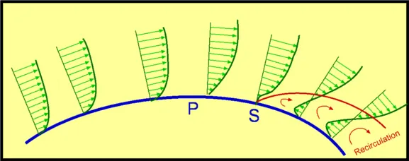
as the fluid flow with a upstream velocity at some distance from the wall of the curved body, that is fluid paricles direction is exactly along the x axis. we can see a convergent divergent flow between the curved body and the upstream velocity. from start point of curved body to point P there is a convergent flow and from point P to end of curved body geometry there is a divergent flow. in the convergent flow th velocity at point P is higher as the area gradually decreases from start point to point P. as the velocity gets increases the pressure gets decreases the from start point to point P. due to this there is a negative pressure gradient developed along the flow. during the flow over a body,the wall shear stress does not allow the fluid to flow along the dirextion due to viscuos effects. but here due to develeoping of negative pressure gradient, the fluid can freely moves over the body by over coming the viscous effects. in the divergnt portion, the area gets increases from point P to end of the geometry. due to this velocity gets decreased and the pressue gets increased which helps in developing of positive pressure gradient. the positive pressure gradient also called adverce presssure gradient.

due to adverce pressure gradient the fluid flows back from end of the body to point P, this flow is called reversal flow. due to the stream line flow and the reversal flow occrs at a region, the fluid particles gets circulated, this is called recirculation. it has been observed that flow is reversed at he vicinity of the wall, this phenomenon is termed as serperation of boundary layer. separation takes place due to excessive momentum loss trying to move downstream againes the adverse pressure gradient. due to separtion of boundary layer, the fluid gets flowed like in the below figure

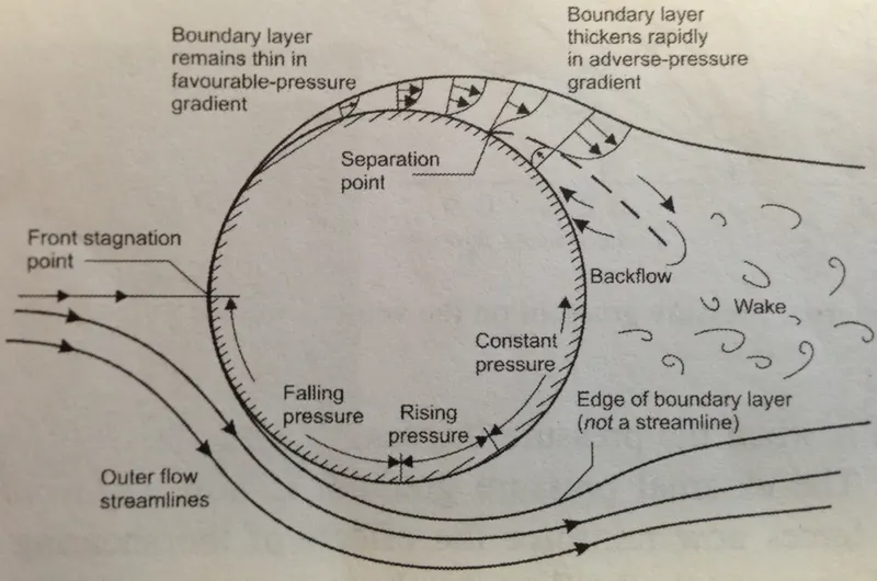
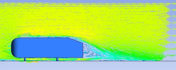
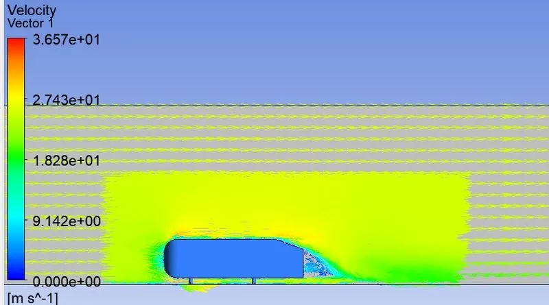
the region where the recirculation of particles occur, that region is called wake region and this region is developed at the rear of th body. the fluid particles at this wake region are very less due to the separation of flow. due to emptiness created in the rear end of the body, then automatically negative pressure gets developed in the rear portion of body.

Simulation of external flow is done here using ansys fluent software. we have to follow the below procedures to simulate the flow.

Geometry:

As the body is perfectly symmetric, we can run the simulation by considering the only half body. This is the best practice where you can save on the number of cells and get the results faster as well.

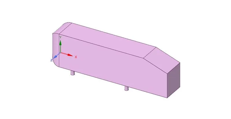
for this symmetric body we are going to prepare domain for the simulation. for this we are going to use enclosure command in the space claim.

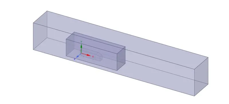
there are two enclosures were used to visualize the simulation results properly . the inner enclosure visualize the wakes developed in the rear end of the ahmed body.

Mesh:

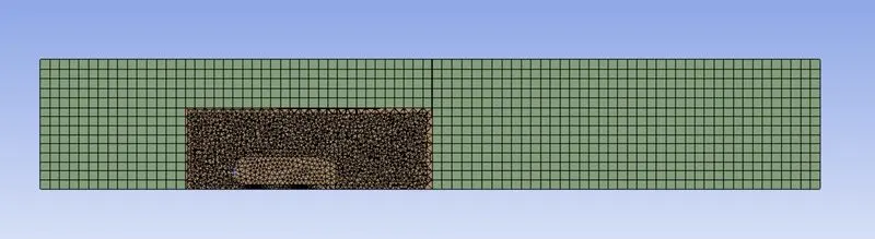
i have used multi zone method for the mesh. the element size of the outer enclosure i have taken as 100mm. the element size of inner enclosure i have taken is 50mm. here the boundaries were named as inlet, outlet, car-wall, symmetry, wall. there are also some inflation layers were created at the wall boundary, that is boundary of ahmed body. you can achieving cell/element stacking in the direction normal to the boundary using a feature called Inflation. Essentially, you can inflate the mesh with several layers from the surface of the boundary until you cover the boundary layer thickness fully. the fist layer thickness is calculated using y+ value.

y+ value-

y+ is a non-dimensional distance. It is important in turbulence modeling to determine the proper size of the cells near domain walls to check if the mesh is fine enough to catch the boundary layer near the walls. the valueof y+ is different for different turbulence models. for k-epsilon standard turbulancee model the y+ value id ranging from 30 to 300, for k-omega SST model the y+ value is rnging from 0 to 5.

to determine the size of the cell at the boundary, that is first layer thickness we have to use below formulae

Firstly, we should calculate the Reynolds number for our model based on the characteristic scales of our geometry such that:

`Re = (rho.U.L)/mu`,

where `rho` and `mu` are the fluid density and viscosity respectively, `U` is the freestream velocity, and L is the characteristic length (e.g. pipe diameter, body length, etc.).

The definition of the y+ value is such that:

`Y+ = (rho. Ut.∆y1)/μ``→ ∆y1=(Y+.μ)/(rho.Ut)`

the frictional velocity, Ut is defined as:

`Ut = √(τ_w/ρ)`

The wall shear stress, `tau_w` can be calculated from skin friction coefficient, `Cf`, such that:

`tau_w = 1/2.Cf.rho.U^2`

for an external flow, the Cf value is defined as:

`Cf = 0.058 * Re^-0.2`

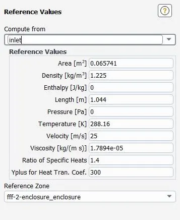
by using the above formulae we can calculate the first layer thickness. here we are taking air as fluid and we are going to take the default values of air from ansys fluent. i am going to use k-omega SST turbulent model for the simulation. so i have taken the value of y+ as 0.1.

for value of y+ = 0.1, the first layer thickness obtained from above formulae is 1.43296646938931E-06 m . by using first layer thickness i have created 6 layers at the boundary with growth rate of 1.2, now there are 115480 cells were generated.

Set up:

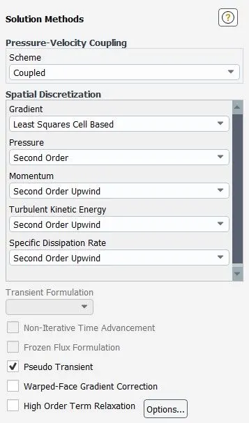
first we have to set up the boundaries. here air is flow over the body with 25m/s, we can say with mach number 0.075. if the mach number is greater than 0.3,we have to consider compressibility effects so we have to use density based solver. if mach number is less than 0.3, we have to use pressure based solver. here i have used pressure based steady state solver.

solver type- pressure based

time-steady state

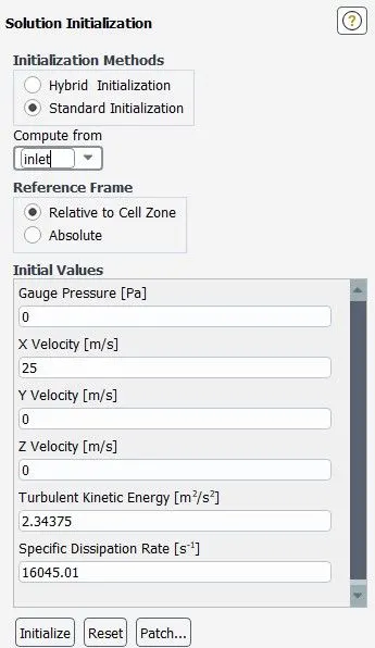
solution:

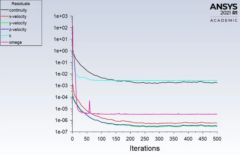
residuals plot-

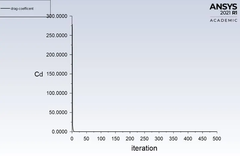
drag coefficent plot-

the coeffeicent of drag obtained here is 0.38798423

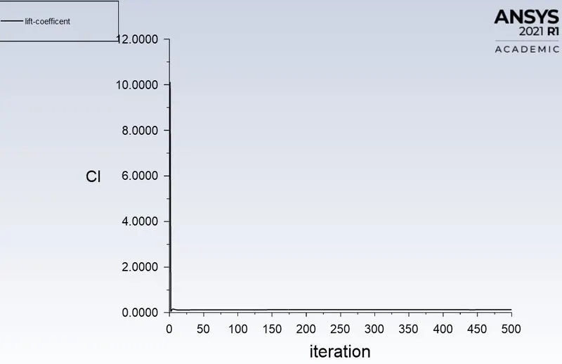
lift coefficent plot-

the lift coefficent obtained here is 0.13161019

result:

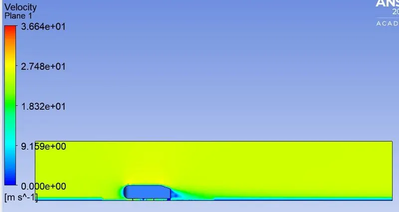
velocity contour plot-

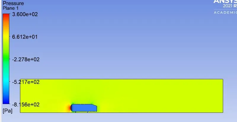
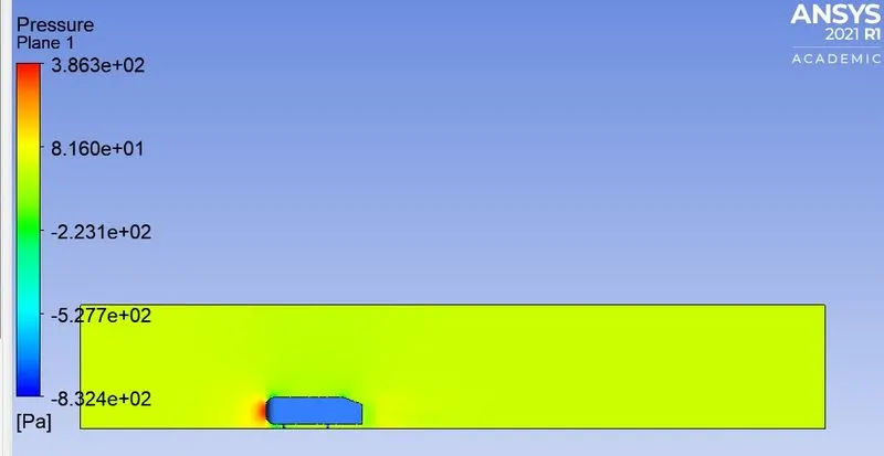
pressure contour plot-

velocity vector plot showing wake region-

grid independency test:

now we use element size as 90mm and the element size of inner enclosure as 28.5mm. the mesh was generated with 496083 cells.

solution:

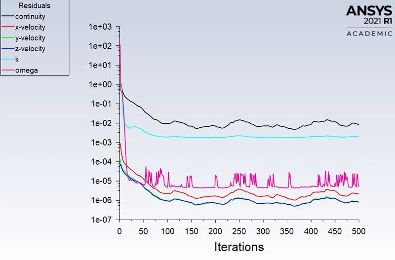
residuals plot-

drag coefficent plot-

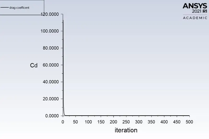
the coefficent of drag obtained is 0.35103457

lift coefficent plot-

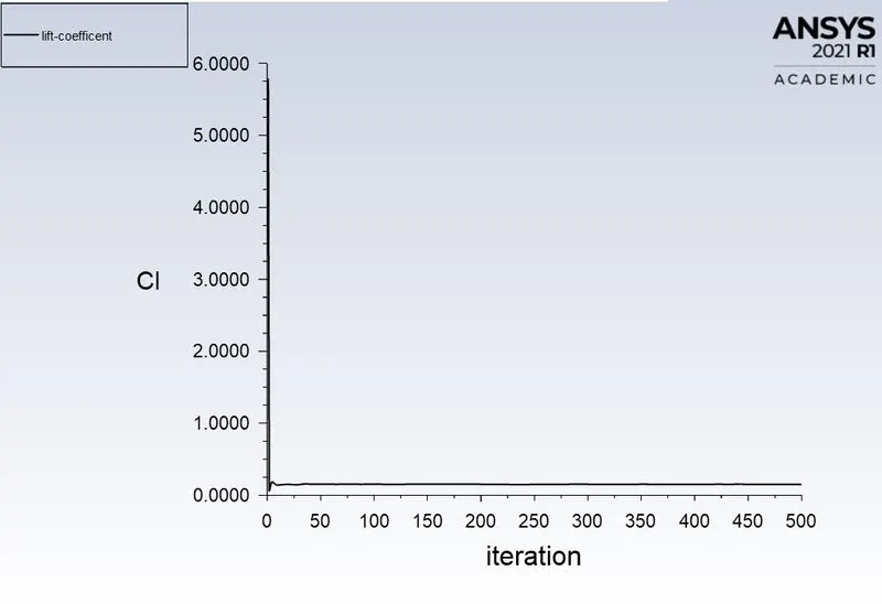
the coefficent of lift obtained is 0.15192873

result:

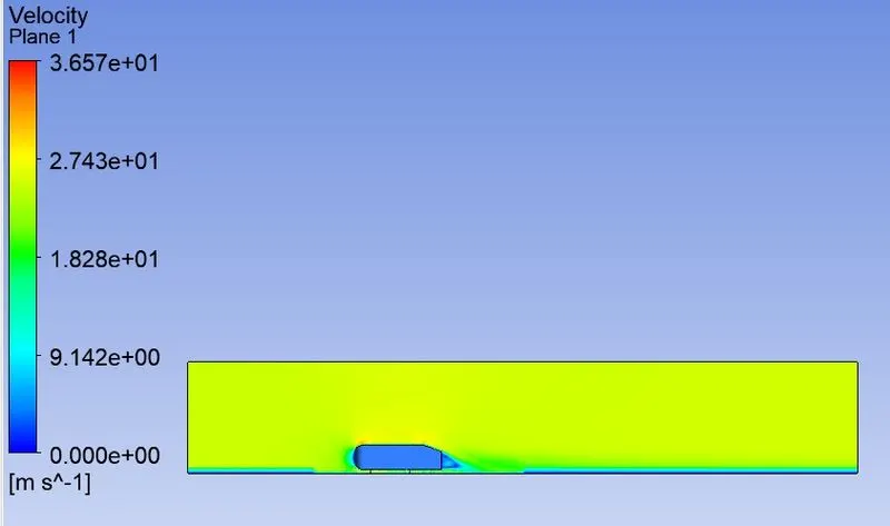
velocity contour-

pressure contour-

velocity vector plot showing wake region-

elements	drag coefficent	lift coefficent
115480	0.38798423	0.13161019
496083	0.35103457	0.15192873

conclusion:

• as the element size of the mesh decreases, we are getting the accurate results.
• with decrease of mesh size, the time taken to calculate the problem is increased.
• by providing inflation layers at the boundary layer of the ahmed body, we can clearly visualize the primitive variables clearly.
• there is a negative pressure is created at the rear part of the ahmed body due to flow separation at the rear end of the body.