Week 11 - Simulation of Flow through a pipe in OpenFoam
AIM:
Simulation of flow through a pipe in OpenFoam
Objectives:
- write code in Matlab to automate the generation of blockMeshDict file.
- Validate Hydro-dynamic length with the numerical result.
- Validate the fully developed flow velocity profile with its analytical profile.
- Validate maximum velocity and pressured drop for fully developed flow.
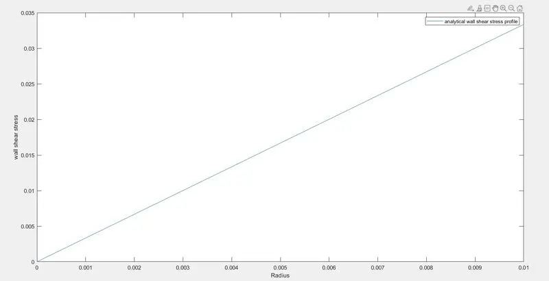
- Post-process Shear stress and validate wall shear stress for fully developed flow
Theory:
consuder a fluid (example:water)flowing through a pipe. the flow in the pipe is incompressible laminar flow with reynolds number 2100.Flow through pipes is an important engineering problem in fluid mechanics. Almost in all our daily operations, we come across pipe flow. For example, the household water supply, sewage flows etc. The pipe flow is also used for the transportation of chemicals and petroleum products in different chemical and oil industries.
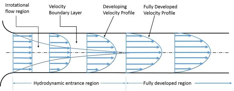
the above figure represents how the fluid is moving along the pipe. intially the fluid enters the ipe with constant velocity. as the fluid enters the pipe, the velocty of the fluid at pip surface is going to be zero due to no slip condition and the velocity of fluid at the centre getting increases. this is beacause of mainatining of the constant mass flow rate at each section in the pipe. the length of the pipe is taken based on the hydrodynamic region length.
Laminar boundary layer:
Laminar boundary-layer flows occur when a moving viscous fluid comes in contact with a solid surface and a layer of rotational fluid, the boundary layer, forms in response to the action of viscosity and the no slip boundary condition on the surface. When the surface is flat or mildly curved and the boundary layer that develops on it is thin and remains adjacent to it, the flow within this layer may be determined by simplifying the Navier-Stokes equations to account for the flow's geometry and then solving the simplified equations.
hydrodynamic entrance length:
Entrance length refers to the length of the entry region, the area following the pipe entrance where effects originating from the interior wall of the pipe propagate into the flow as an expanding boundary layer. When the boundary layer expands to fill the entire pipe, the developing flow becomes a fully developed flow, where flow characteristics no longer change with increased distance along the pipe. Many different entrance lengths exist to describe a variety of flow conditions. Hydrodynamic entrance length describes the formation of a velocity profile caused by viscous forces propagating from the pipe wall.
to calculate the pressure drop and wall shear stress in the pipe, we have to use hagen poiseuille equation. the below formulae are obtained from hagen poiseuille equation.
- pressure drop along the length of the pipe, `∆P= (32μVL)/D^2`
- average velocity in the pipe, `V = (Re*μ)/D`
- wall shear stress , `τ= (16*μ*V*R)/(D^2)`
- hydrodynamic entrance length for laminar flow is `Le = 0.06*Re*D`
- length of the pipe,`L = Le+0.48` (note:we can take the length can be any value greater than hydrodynamic entrance length.)
where μ is the kinematic viscosity, D is the diamter of the pipe, Re is the reynolds number.
Constant values in the pipe flow:
fluid : water
dynamic viscosity of water = 8.89*`10^-4 (NS)/m^2`
Reynolds number, Re = 2100
density of water = `997 (kg)/m^3`
kinematic viscosity = dynamic viscosity/density = 8.926*`10^-7 (m^2)/S`
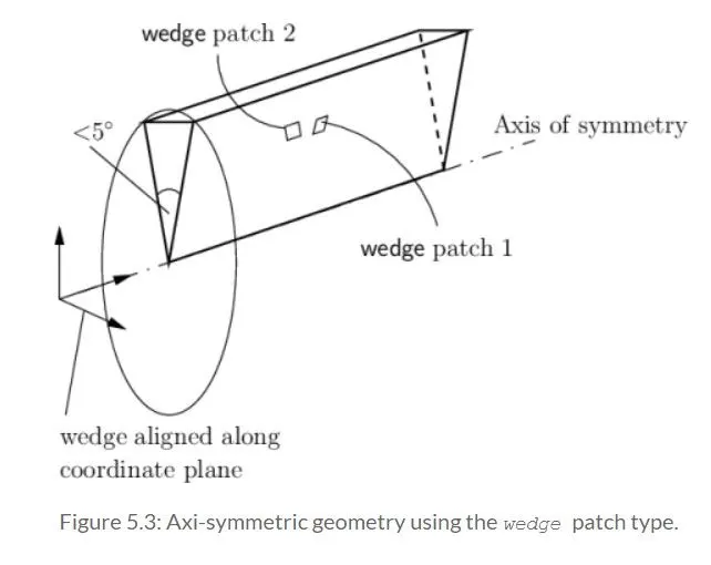
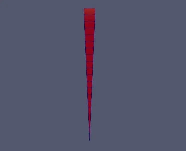
here we are taking a wedge in the pipe. for that part we are going to simulate the flow.we can equate the output of these simulations as the output of the entire flow in the pipe, because wedge is axi symmetric in nature with pipe. OpenFOAM is designed as a code for 3-dimensional space and defines all meshes as such. However, 1- and 2- dimensional and axi-symmetric problems can be simulated in OpenFOAM by generating a mesh in 3 dimensions and applying special boundary conditions on any patch in the plane(s) normal to the direction(s) of interest. More specifically, 1- and 2- dimensional problems use the empty patch type and axi-symmetric problems use the wedge patch type.
block representation:
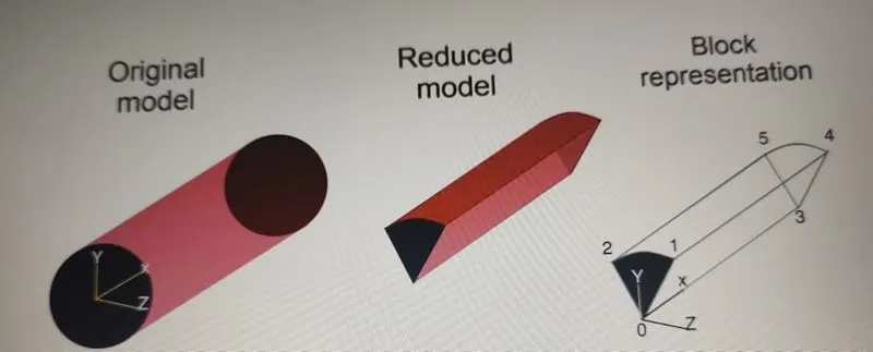
we have to take wedge angle less than or equal to 5 degrees. because taking of 5 degree is enough to tell that the shape is circular. by increasing the wedge angle greater than 5, the size of the cell will increase then errors gets increased.
first we have to write mat lab programme for hagen poiseuille equation to get the analytical values of above formulae. and then we are going to generate the blockMeshDict file in the matlab.
matlab main function:
clear all
close all
clc

%inputs
%diamter of pipe(m)
D = 0.02;
%wedge angle
theta = 5;
%reynolds number
Re = 2100;
%entrance length
Le = 0.06*Re*D;
%length of pipe
L = 3;
%dynamic viscosity of water(NS/m^2)
dynamic_viscosity = 8.9e-4;
%density(kg/m^3)
rho = 997;
%kinematic viscosity(m^2/S)
mu = dynamic_viscosity/rho;
%average_velocity(m/s)
V = Re*mu/D;
%maximum velocity
V_max = 2*V;
%kinematic pressure drop(N/m^2)
delta_p = 32*mu*V*L/D^2;
%radius
R = linspace(0,0.01,20);

for i = 1:length(R)
    %local velocity
    V_local(i) = 2*V*(1-(4*R(i)^2/D^2));

    %wall shear stress
    tau(i) = 16*mu*rho*V*R(i)/D^2;
end
% figure(1)
% plot(R,V_local)
% xlabel('Radius')
% ylabel('local velocity')
% legend('analytical velocity profile')
%
% figure(2)
% plot(R,tau)
% xlabel('Radius')
% ylabel('wall shear stress')
% legend('analytical wall shear stress profile')

%BlockMeshdict file:
%vertices
v_0 = [0 0 0];
v_1 = [0 D/2*cosd(theta/2) D/2*sind(theta/2)];
v_2 = [0 D/2*cosd(theta/2) -D/2*sind(theta/2)];
v_3 = [L 0 0];
v_4 = [L D/2*cosd(theta/2) D/2*sind(theta/2)];
v_5 = [L D/2*cosd(theta/2) -D/2*sind(theta/2)];

%headers
h1 = '/*--------------------------------*- C++ -*----------------------------------*';
h2 = '  =========                 |';
h3 = '  \      /  F ield         |';
h4 = '   \    /   O peration     |';
h5 = '    \  /    A nd           |';
h6 = '     \/     M anipulation  |';
h7 = '*---------------------------------------------------------------------------*/';
%creating blockmeshdict file
f1 = fopen('blockMeshDict.text','w');

fprintf(f1, '%sn', h1)
fprintf(f1, '%sn', h2)
fprintf(f1, '%sn', h3)
fprintf(f1, '%sn', h4)
fprintf(f1, '%sn', h5)
fprintf(f1, '%sn', h6)
fprintf(f1, '%sn', h7)
fprintf(f1, 'FoamFilen%sn','{')
fprintf(f1, '%10s %13sn', 'version', '2.0;')
fprintf(f1, '%9s %16sn', 'format', 'ascii;')
fprintf(f1, '%8s %22sn', 'class', 'dictionary;')
fprintf(f1, '%9s %24sn', 'object', 'blockMeshDict;')
fprintf(f1, '%sn','}')
h8 = '// * * * * * * * * * * * * * * * * * * * * * * * * * * * * * * * * * * * * * //';
fprintf(f1, '%sn',h8)
fprintf(f1, '%s %5sn', 'convertToMeters', '1;')

fprintf(f1, 'verticesn%sn','(')
fprintf(f1, 't(%d %d %d)n',v_0)
fprintf(f1, 't(%d %d %d)n',v_1)
fprintf(f1, 't(%d %d %d)n',v_2)
fprintf(f1, 't(%d %d %d)n',v_3)
fprintf(f1, 't(%d %d %d)n',v_4)
fprintf(f1, 't(%d %d %d)n',v_5)
fprintf(f1, '%sn',');')

fprintf(f1, 'blocksn%sn','(')
fprintf(f1, 'thex (0 3 5 2 0 3 4 1)(200 20 1)')
fprintf(f1, ' simpleGrading (0.2 1 1)n);n')

fprintf(f1, 'edgesn%sn', '(')
fprintf(f1, 'tarc 1 2 (%d %d %d)n', 0,D/2,0)
fprintf(f1, 'tarc 4 5 (%d %d %d)n);n', L,D/2,0)

fprintf(f1, 'boundaryn')
fprintf(f1,'%sn','(')
fprintf(f1, 'tinletn')
fprintf(f1, 't{n')
fprintf(f1, '%15s %6sn', 'type', 'patch;')
fprintf(f1, '%16sn%12sn', 'faces','(')
fprintf(f1, 'tt(0 1 2 0)n')
fprintf(f1, '%12sn',');')
fprintf(f1, 't}n')
fprintf(f1, 'toutletn')
fprintf(f1, 't{n')
fprintf(f1, '%15s %6sn', 'type', 'patch;')
fprintf(f1, '%16sn%12sn', 'faces','(')
fprintf(f1, 'tt(3 5 4 3)n')
fprintf(f1, '%12sn',');')
fprintf(f1, 't}n')
fprintf(f1, 'ttopn')
fprintf(f1, 't{n')
fprintf(f1, '%15s %6sn', 'type', 'wall;')
fprintf(f1, '%16sn%12sn', 'faces','(')
fprintf(f1, 'tt(4 5 2 1)n')
fprintf(f1, '%12sn',');')
fprintf(f1, 't}n')
fprintf(f1, 'tfrontn')
fprintf(f1, 't{n')
fprintf(f1, '%15s %6sn', 'type', 'wedge;')
fprintf(f1, '%16sn%12sn', 'faces','(')
fprintf(f1, 'tt(0 3 4 1)n')
fprintf(f1, '%12sn',');')
fprintf(f1, 't}n')
fprintf(f1, 'tbackn')
fprintf(f1, 't{n')
fprintf(f1, '%15s %6sn', 'type', 'wedge;')
fprintf(f1, '%16sn%12sn', 'faces','(')
fprintf(f1, 'tt(0 2 5 3)n')
fprintf(f1, '%12sn',');')
fprintf(f1, 't}n')
fprintf(f1, 'taxisn')
fprintf(f1, 't{n')
fprintf(f1, '%15s %6sn', 'type', 'empty;')
fprintf(f1, '%16sn%12sn', 'faces','(')
fprintf(f1, 'tt(0 3 3 0)n')
fprintf(f1, '%12sn',');')
fprintf(f1, 't}n')
fprintf(f1, ');n')

fprintf(f1, 'mergePatchPairsn')
fprintf(f1, '(n);n')
h9 = '// ************************************************************************* //';
fprintf(f1,'%s',h9)

fclose(f1)
blockmeshdict file in openFoam:
/*--------------------------------*- C++ -*----------------------------------*
  =========                 |
        /  F ield         | OpenFOAM: The Open Source CFD Toolbox
       /   O peration     | Website:  https://openfoam.org
      /    A nd           | Version:  dev
     /     M anipulation  |
*---------------------------------------------------------------------------*/
FoamFile
{
    version     2.0;
    format      ascii;
    class       dictionary;
    object      blockMeshDict;
}
// * * * * * * * * * * * * * * * * * * * * * * * * * * * * * * * * * * * * * //

convertToMeters 1;

vertices
(
    (0 0 0)
    (0 9.990482e-03 4.361939e-04)
    (0 9.990482e-03 -4.361939e-04)

    (3 0 0)
    (3 9.990482e-03 4.361939e-04)
    (3 9.990482e-03 -4.361939e-04)
);

blocks
(
    hex (0 3 5 2 0 3 4 1) (250 50 1) simpleGrading (1 0.2 1)
);

edges
(
    arc 1 2 (0 1.000000e-02 0)
    arc 4 5 (3 1.000000e-02 0)
);

boundary
(
    inlet
    {
        type patch;
        faces
        (
            (0 1 2 0)
        );
    }
    outlet
    {
        type patch;
        faces
        (
            (3 5 4 3)
        );
    }
    top
    {
        type wall;
        faces
        (
            (4 5 2 1)
        );
    }
    front
    {
         type wedge;
         faces
         (
            (0 3 4 1)
         );
     }
     back
     {
          type wedge;
          faces
          (
             (0 2 5 3)
          );
     }
     axis
     {
         type empty;
         faces
         (
            (0 3 3 0)
         );
      }
);

mergePatchPairs
(
);

// ************************************************************************* //
controldict file:
/*--------------------------------*- C++ -*----------------------------------*
  =========                 |
        /  F ield         | OpenFOAM: The Open Source CFD Toolbox
       /   O peration     | Website:  https://openfoam.org
      /    A nd           | Version:  dev
     /     M anipulation  |
*---------------------------------------------------------------------------*/
FoamFile
{
    version     2.0;
    format      ascii;
    class       dictionary;
    location    "system";
    object      controlDict;
}
// * * * * * * * * * * * * * * * * * * * * * * * * * * * * * * * * * * * * * //

application     icoFoam;

startFrom       startTime;

startTime       0;

stopAt          endTime;

endTime         50;

deltaT          0.01;

writeControl    timeStep;

writeInterval   100;

purgeWrite      0;

writeFormat     ascii;

writePrecision  6;

writeCompression off;

timeFormat      general;

timePrecision   6;

runTimeModifiable true;


// ************************************************************************* //
the initial boundary conditions we use in simulating the flow is inlet velocity and outlet pressure.
the inlet velocity is obtained from the above formulae
inlet veocity,V = 8.926*2100*`10^-7``/0.02` = 0.09373`m/s`
pressure:
/*--------------------------------*- C++ -*----------------------------------*
========= |
 / F ield | OpenFOAM: The Open Source CFD Toolbox
 / O peration | Website: https://openfoam.org
 / A nd | Version: dev
/ M anipulation |
*---------------------------------------------------------------------------*/
FoamFile
{
version 2.0;
format ascii;
class volScalarField;
object p;
}
// * * * * * * * * * * * * * * * * * * * * * * * * * * * * * * * * * * * * * //

dimensions [0 2 -2 0 0 0 0];

internalField uniform 0;

boundaryField
{
inlet
{
type zeroGradient;
}

outlet
{
type fixedValue;
value uniform 0.20079;
}

top
{
type zeroGradient;
}

front
{
type wedge;
}

back
{
type wedge;
}

axis
{
type empty;
}
}

// ************************************************************************* //
velocity:
/*--------------------------------*- C++ -*----------------------------------*
  =========                 |
        /  F ield         | OpenFOAM: The Open Source CFD Toolbox
       /   O peration     | Website:  https://openfoam.org
      /    A nd           | Version:  dev
     /     M anipulation  |
*---------------------------------------------------------------------------*/
FoamFile
{
    version     2.0;
    format      ascii;
    class       volVectorField;
    object      U;
}
// * * * * * * * * * * * * * * * * * * * * * * * * * * * * * * * * * * * * * //

dimensions      [0 1 -1 0 0 0 0];

internalField   uniform (0 0 0);

boundaryField
{
    inlet
    {
        type            fixedValue;
        value           uniform (0.9373 0 0);
    }

    outlet
    {
        type            zeroGradient;
    }

    top
    {
        type            noSlip;
    }

    front
    {
        type            wedge;
    }

    back
    {
        type            wedge;
    }

    axis
    {
        type            empty;
    }
}

// ************************************************************************* //
result:
after running the code
wedge of the pipe with angle 5 degrees
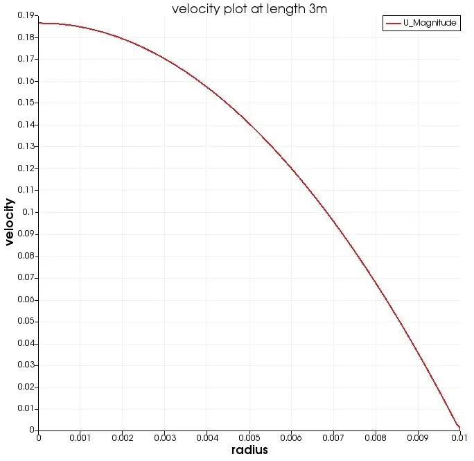
the velocity plot at length 3m:
the velocity profile at hydrodynamic length(2.52m):
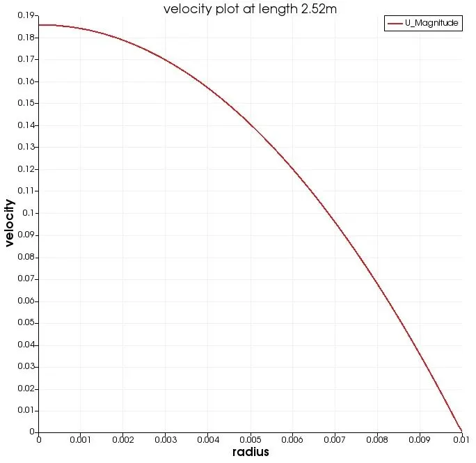
the velocity profile at the length 3m is same as at hydrodyamic length 2.52m. because in the fully developed zone the velocity profile is same at every point.
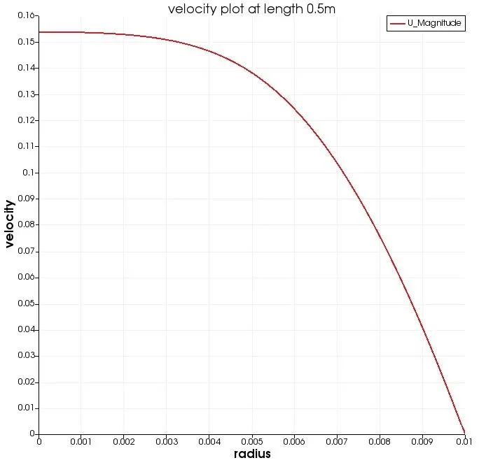
velocity profile at 0.5m, that is in the hydrodynamic region:
the below plot is the analytical velocity profile obtained from the matlab at length 3m.
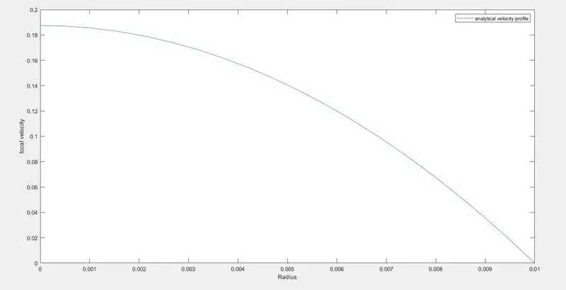
by comparing the both the velocity profiles obtained from matlab and openfoam at length 3m . the maximum velocity obtained from the matlab is 0.1875 m/s where as the actual maximum velocity otained is 0.1865m/s. the error is 0.001.
the pressure plot:
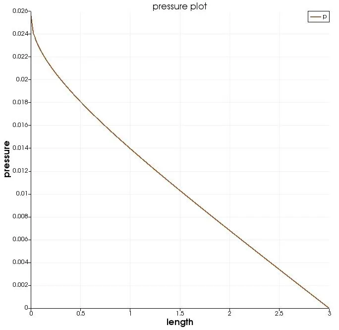
the pressure drop from the ebove plot is 0.0256 where as the pressure drop obtained from the hagen poiseuille is 0.0201. the error is 0.0055.
wall shear stress plot:
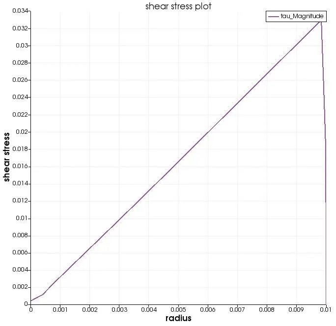
the analytical wall shear stress plot from the matlab is