Week 8: Literature review RANS derivation and analysis

AIM:

Literature review RANS derivation and analysis

Ojectives:

• Explain your understanding of the terms reynold's stress
• What is turbulent viscosity? How is it different from molecular viscosity?

Reynolds stress:

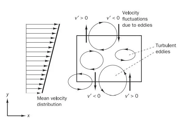
consider a control volume in a two-dimensional turbulent shear flow parallel to the x-axis with a mean velocity gradient in the y-direction in the below figure. The presence of vortical eddy motions creates strong mixing. Random currents that are associated with the passage of eddies near the boundaries of the control volume transport fluid across its boundaries. These recirculating fluid motions cannot create or destroy mass, but fluid parcels transported by the eddies will carry momentum and energy into and out of the control volume. below figure shows that, because of the existence of the velocity gradient, fluctuations with a negative y-velocity will generally bring fluid parcels with a higher x-momentum into the control volume across its top boundary and will also transport control volume fluid to a region of slower moving fluid across the bottom boundary. Similarly, positive y-velocity fluctuations will – on average – transport slower moving fluid into regions of higher velocity. The net result is momentum exchange due to convective transport by the eddies, which causes the faster moving fluid layers to be decelerated and the slower moving layers to be accelerated. Consequently, the fluid layers experience additional turbulent shear stresses, which are known as the Reynolds stresses.

Reynolds-averaged Navier Stokes equations for incompressible flow:

Let us consider a single point measurement in a turbulent flow, e.g. a velocity measurement made with a hot-wire anemometer or a local pressure measurement made with a small transducer. In the belwo figure , we can see that the appearance of turbulence manifested itself as random fluctuations of the measured velocity component about a mean value. All other flow variables, i.e. all other velocity components, the pressure, temperature, density etc.,will also exhibit this additional time-dependent behaviour.

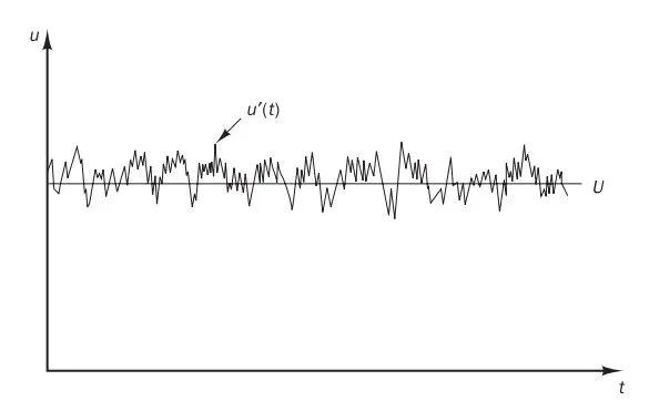
The Reynolds decomposition defines flow property `phi` at this point as the sum of a steady mean component `phi` and a time varying fluctuating component `phi'(t)` with zero mean value: hence

`phi(t) = phi+phi'(t)`

mean of the flow property is defines as

`phi=1/(∆t) ∫_0^(∆t)ϕ(t)dt`

we should take the limit of time interval ∆t approaching infinity, but the process indicated by above equation gives meaningful time averages if ∆t is larger than the time scale associated with the slowest variations (due to large eddies) of property ϕ. This definition of the mean of a flow
property is adequate for steady mean flows. In time-dependent flows the mean of a property at time t is taken to be the average of the instantaneous values of the property over a large number of repeated identical experiments. the so-called ‘ensemble average’.

now i will use this mean flow properties in naviour stokes equation.

first write the reynolds decomposition of velocities

`u(x,y,z,t)=baru(x,y,z)+u’(x,y,z,t)`

`v(x,y,z,t)=barv(x,y,z)+v’(x,y,z,t)`

`w(x,y,z,t)=barw(x,y,z)+w’(x,y,z,t)`

mean of the velocities are

`baru(x,y,z)=1/(∆t )∫_0^(∆t)u(x,y,z,t).dt`

`barv(x,y,z)=1/(∆t )∫_0^(∆t)v(x,y,z,t).dt`

`barw(x,y,z)=1/(∆t )∫_0^(∆t)w(x,y,z,t).dt`

we know that mean time integrral of fluctuation is always zero. for the proof i will integrate the reynold decomposition of u velocity.

`1/(∆t )∫_0^(∆t)u(x,y,z,t).dt=1/(∆t )∫_0^(∆t)baru(x,y,z).dt+ 1/(∆t )∫_0^(∆t)u'(x,y,z,t).dt`

thetime integral of velocity is the mean velocity and the mean velocity is not a function of time so . we can say that `1/(∆t )∫_0^(∆t)u(x,y,z,t).dt=1/(∆t )∫_0^(∆t)baru(x,y,z).dt`

so finall we can say that `1/(∆t )∫_0^(∆t)u'(x,y,z,t).dt = 0`

now taken contiuety equation and them incert reynolds decomposition terms

`(∂u)/(∂x)+(∂v)/(∂y)=0`

`(∂(baru+u^'))/(∂x)+(∂(barv+v^'))/(∂y)=0`

now integrste the equation with respect to time and do time averaging

`1/(∆t )∫_0^(∆t )∂(baru+u^' )/(∂x) dt+∂(barv+v^' )/(∂y) dt=0`

`1/(∆t) ∫_0^(∆t)(∂baru)/(∂x) dt+1/(∆t) ∫_0^(∆t)(∂u')/(∂x) dt+1/(∆t) ∫_0^(∆t)(∂barv)/(∂y) dt+1/(∆t )∫_0^(∆t)(∂v')/(∂y) dt=0`

we know that the time average of fluctuation terms are zeros. so the derivatives of the fluctions also be zero. so the final equation is

`1/(∆t) ∫_0^(∆t)(∂baru)/(∂x) dt+1/(∆t) ∫_0^(∆t)(∂barv)/(∂y) dt=0`

`(∂baru)/(∂x) +(∂barv)/(∂y) = 0`

so the continuity equation is satisfied here.

x-momentum equation:

`(∂u)/(∂t)+u (∂u)/(∂x)+v (∂u)/(∂y)=1/ρ ((-∂p)/(∂x))+ν (∂^2u)/(∂y^2)`

where ν is kinematic viscosity.

now add continuity eqyation to LHS so that we can solve the equations smoothly.

`(∂u)/(∂t)+u (∂u)/(∂x)+v (∂u)/(∂y)+u((∂u)/(∂x) +(∂v)/(∂y))=1/ρ ((-∂p)/(∂x))+ν (∂^2u)/(∂y^2)`

by solving this finally we get below equation

`(∂u)/(∂t)+ (∂u^2)/(∂x)+∂(uv)/(∂y)=1/ρ ((-∂p)/(∂x))+ν (∂^2u)/(∂y^2)`

now integrating with respect to time and do time averaging and incert reynolds decomposition terms

`1/(∆t) ∫_0^(∆t)`

`1/(∆t) ∫_0^(∆t)(∂(baru+u'))/(∂t)+ (∂(baru+u')^2)/(∂x)+∂((baru+u')(barv+v'))/(∂y)=1/(∆t) ∫_0^(∆t)1/ρ ((-∂(barp+p'))/(∂x))+ν (∂^2(baru+u'))/(∂y^2)`

now after cancelling the fluctuationg terms finally we get the below equation

`1/(∆t) ∫_0^(∆t)(∂baru)/(∂t) dt+1/(∆t) ∫_0^(∆t)(∂baru^2)/(∂x) dt+1/(∆t) ∫_0^(∆t)(∂(baru.barv))/(∂x) dt+1/(∆t) ∫_0^(∆t)(∂(u'.v'))/(∂x) dt=1/ρ ((-∂barp)/(∂x))+ν (∂^2baru)/(∂y^2)`

we can not cancel the fluction term u'.v' because the as the fluid moves there is a positive fluction of velocity along y axis and negative fluctuation along x axis. so the final fluctuation will also be a negative value which is non zero value.

the final obtained equation is

`(∂baru)/(∂t)+ (∂baru^2)/(∂x)+∂(baru.barv)/(∂y)=1/ρ ((-∂barp)/(∂x))+ν (∂^2baru)/(∂y^2)+1/(∆t) ∫_0^(∆t)(∂(u'.v'))/(∂x) dt`

final Renolds averaged navior stokes equation is

`ρ((∂baru)/(∂t)+ (∂baru^2)/(∂x)+∂(baru.barv)/(∂y))= ((-∂barp)/(∂x))+μ (∂^2baru)/(∂y^2)-ρ/(∆t) ∫_0^(∆t)(∂(u'.v'))/(∂x) dt`

where μ is absolute viscosity

`μ (∂^2baru)/(∂y^2)`is viscous stress

`ρ/(∆t) ∫_0^(∆t)(∂(u'.v'))/(∂x) dt` is reynolds stress

• the most common approach to calclulate reynolds stress is Boussinesq hypothesis

Prior to the application of numerical methods the Navier–Stokes equations are time averaged (or ensemble averaged in flows with time-dependent boundary conditions). Extra terms appear in the time-averaged (or Reynolds averaged) flow equations due to the interactions between various turbulent fluctuations. These extra terms (turbulence viscosity) are modelled with classical turbulence models such as k-omega, k- epsilon modets etc..

turbulent viscosity(eddy ciscosity):

The turbulent trasfer of momentum by eddies giving rise to an internal fluid friction, in a manner analogous to the action of molecular viscosity in laminar flow, but taking place on a much larger scale. Eddy viscosity is a function of the flow, not of the fluid. It is greater for flows with more turbulence. The value of the coefficent of eddy viscosity is of the order of 1 m² s^-1

molecular viscosity:

At a molecular level, viscosity is a result the interaction between the different molecules in a fluid. This can be also understood as friction between the molecules in the fluid. Just like in the case of friction between moving solids, viscosity will determine the energy required to make a fluid flow.molecular viscosity is also termed as asolute viscosity.

how turbulent viscosity differ from molecular viscosity:

• molecular viscosity exists due to interactions between the fluid partilcles in which friction is present between the fluid particles where as the turbulent viscosity present due to eddies formed due to turbulence of flow.
• generally molecular viscosity is seen in laminar flow but we can't see turbulent viscosity in laminar flow because there won't be any fluctuations of primitive variables which can be seen in turbulent flows.