Week 3: Flow over a backward facing step

AIM:

Flow over a backward facing step

objectives:

run the case for three different base mesh sizes

• dx = dy = dz =2e-3 m
• dx = dy = dz =1.5e-3 m
• dx = dy = dz =1.0e-3 m

Contents to be shown in the report-

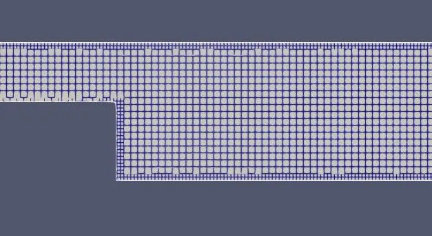
1. Show the mesh (i.e surface with edges) for all the 3 base mesh sizes

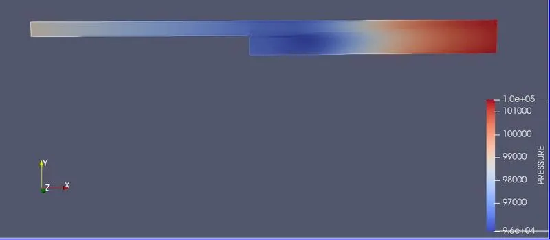
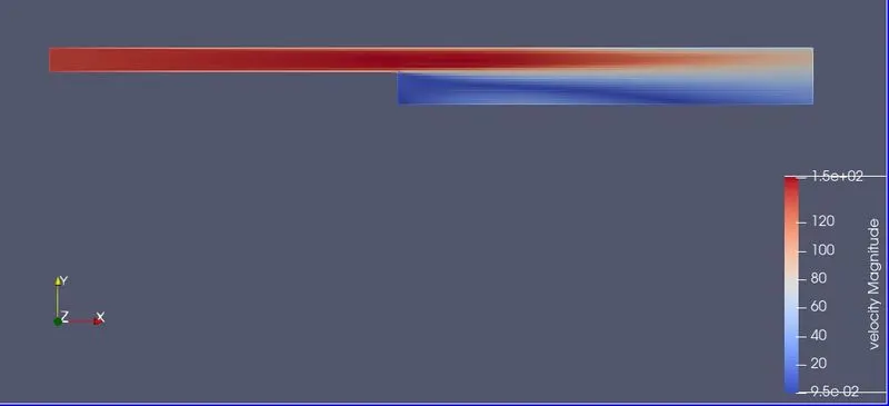
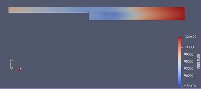
2.Show pressure and velocity contours

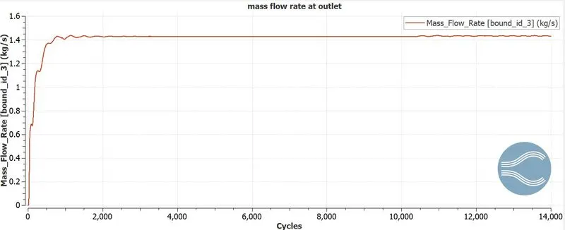
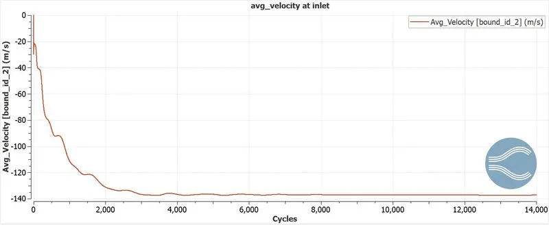
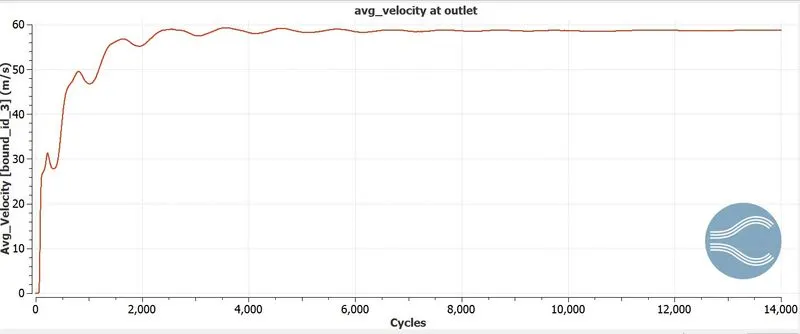
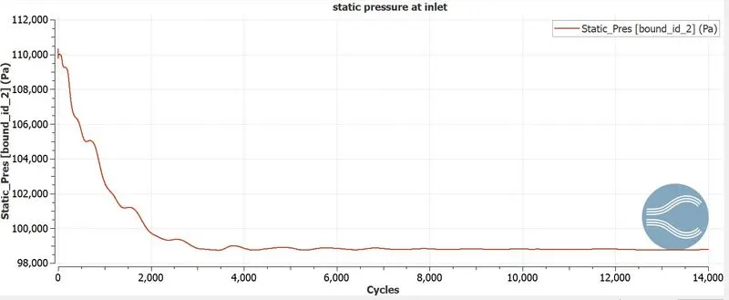
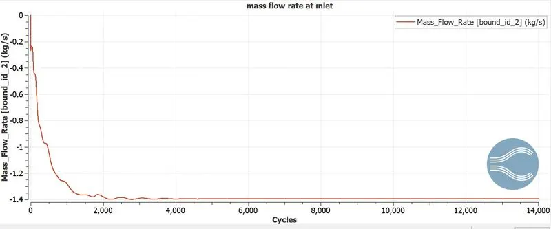
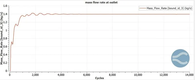
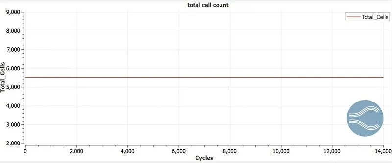
3. Show the plots of velocity, pressure, mass flow rate and total cell count for all the 3 base mesh sizes

4. Also explain where and why separation is taking place in detail.

theory:

Many industrial application involves flow separation and reattachment. To illustrate this phenomenon, flow simulation over backward facing step is considered.Fully developed flow enters the domain from left. When the flow reaches the step, because of expansion of flow channel, pressure gradient exists, it detaches and a recirculation zone is formed. A turbulent boundary layer encounters a sudden back step, causing flow separation. Later the flow eventually reattaches to the bottom wall.

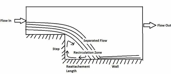
explain where and why separation is taking place in detail:

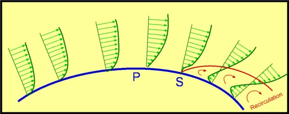
as the fluid flow with a upstream velocity at some distance from the wall of the curved body, that is fluid paricles direction is exactly along the x axis. we can see a convergent divergent flow between the curved body and the upstream velocity. from start point of curved body to point P there is a convergent flow and from point P to end of curved body geometry there is a divergent flow. in the convergent flow th velocity at point P is higher as the area gradually decreases from start point to point P. as the velocity gets increases the pressure gets decreases the from start point to point P. due to this there is a negative pressure gradient developed along the flow. during the flow over a body,the wall shear stress does not allow the fluid to flow along the dirextion due to viscuos effects. but here due to develeoping of negative pressure gradient, the fluid can freely moves over the body by over coming the viscous effects. in the divergnt portion, the area gets increases from point P to end of the geometry. due to this velocity gets decreased and the pressue gets increased which helps in developing of positive pressure gradient. the positive pressure gradient also called adverce presssure gradient.

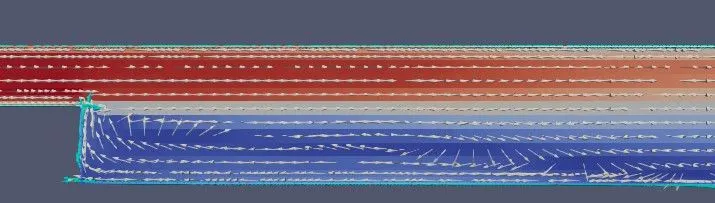
due to adverce pressure gradient the fluid flows back from end of the body to point P, this flow is called reversal flow. due to the stream line flow and the reversal flow occrs at a region, the fluid particles gets circulated, this is called recirculation. it has been observed that flow is reversed at he vicinity of the wall, this phenomenon is termed as serperation of boundary layer (boundary layer separation). separation takes place due to excessive momentum loss trying to move downstream againes the adverse pressure gradient.

to do the simulation i have used convegence software.

geometry:

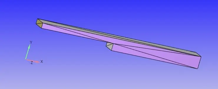
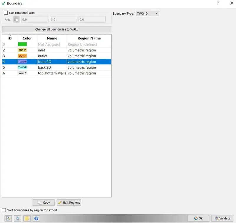
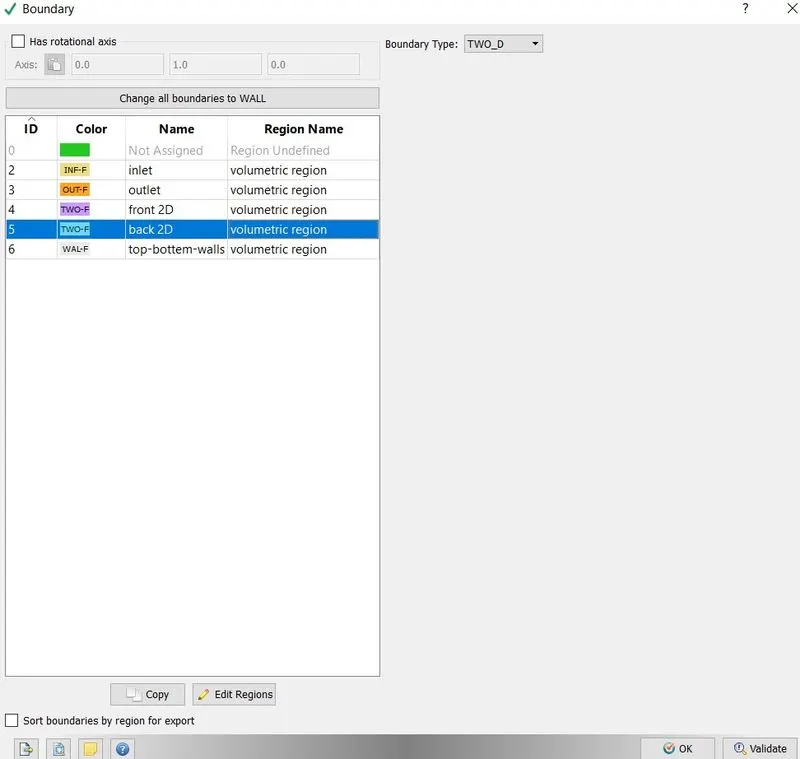
now check the normals of all the faces are facing inside or not by using normal toggle tool and then buid case setup.then i have used boundary tool in the geometry. here i have named the boundaries to the box. i have named the front and back as 2D because i have i have taken the geoemtry to be 2D geometry. i am considering the 2D geometry because the channel length along z axis is infinite. so we can take any plane normal to z axis, it shows the same results at every plane. i have taken xy plane

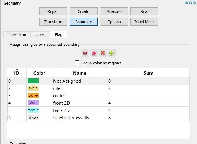
in the above figure, sum represents the number of triangles selected at the each boundary. now use normal toggle tool. in the converge,the normals are aloways directed to outside of the box faces as a default. but here the fluid is inward flow. so eliminate them, click on transform in geometry and slect of triangle and click apply. to check whethere the geometry is correct or not(ie open edges errors, overlap errors), click on the diagnosis which is shown at the bottem left of the display and click findings. mow buid the case setup.

case setup:

application type: time beased

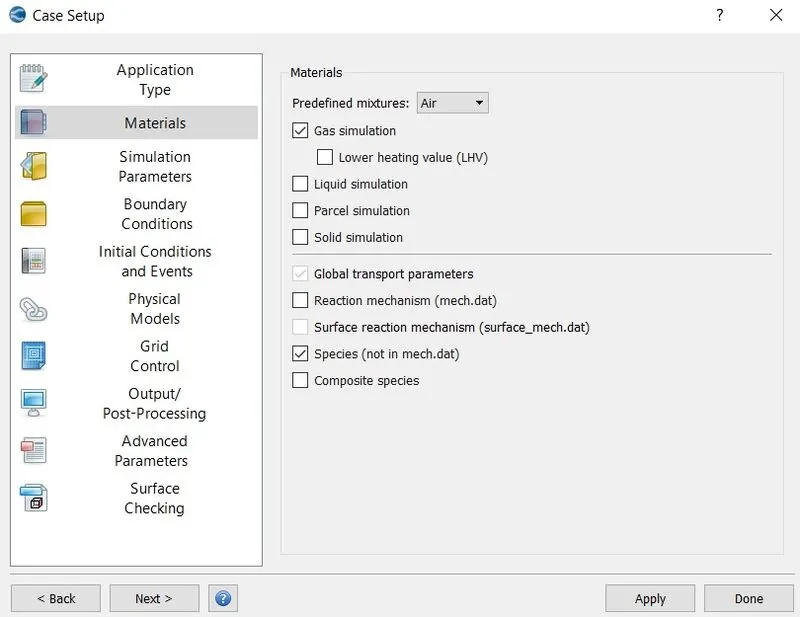
materials: air

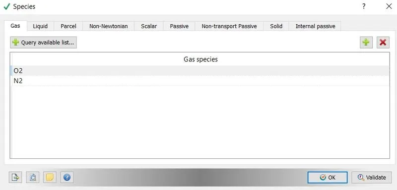
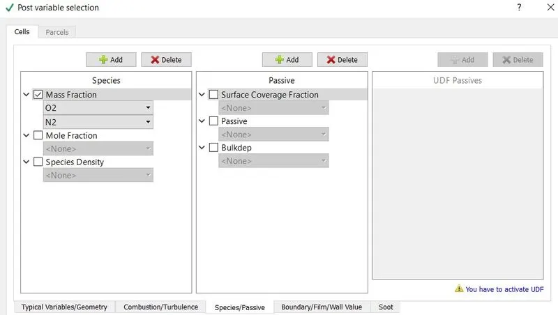
click on gas simulation as the air is gaseous state and click on species to calcuate how the mass fraction of N2 and O2 are changing along the flow.

species-

simulation parameters:

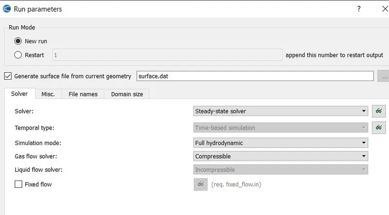
run parameters-

i am running the somulation using steady state solver. full hydrodynamic simulation mode is used for simple geometries.

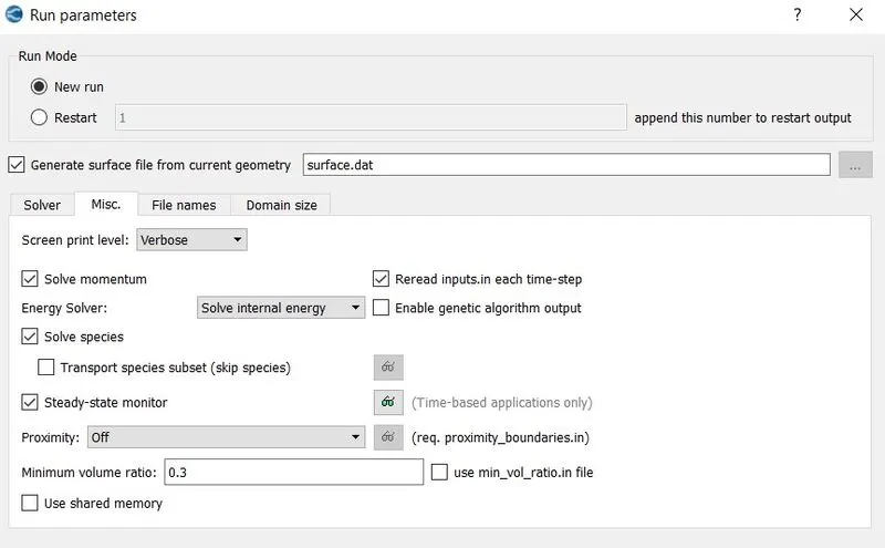
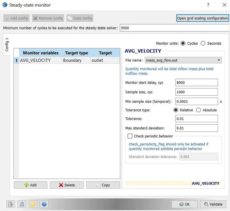
• steady state moniter- it moniters the primitive variables wheather they reached the steady state or not. minimum number of cycles to be executed for steady state solver is 5000. it tells that even if we give the number of cycles to run the simulation at 15000, the software stop calculating the simulation if it reached the steady state in between 5000 and 15000 cycles. moniter start delay indicates the the software start monitoring the simulation whether the solution reached to steady state or not., that is from start. simple size indicates the soft ware takes the solution for every 1000 cycles and compar the difference in changing of primitive varisbles to see whether they reached steady state or not.tolerence denotes the diference in changing of primitive variables at every 1000cycles.

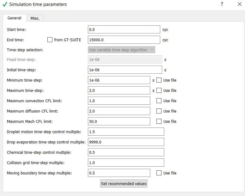
simulation time parameters- the maximum convection cfl number should always be less than or equal to 1. so that solution would converge otherwise solution gets blown up.

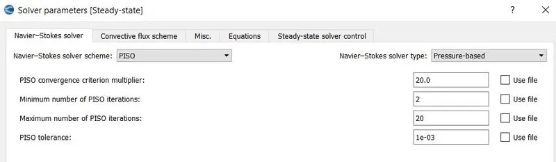
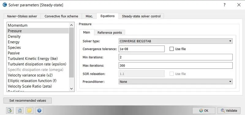
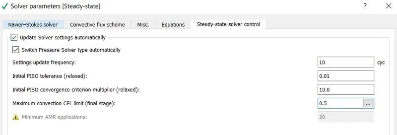
solver parameters-

pressure based solver is used here and the max. cfl number taken is 0.5

initial conditions and events:

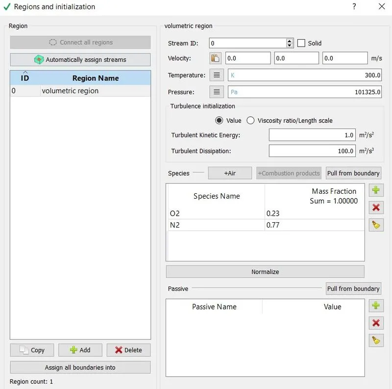
regions and initialization-

here i have named the entire box region as volumetric region.

boundary conditions:

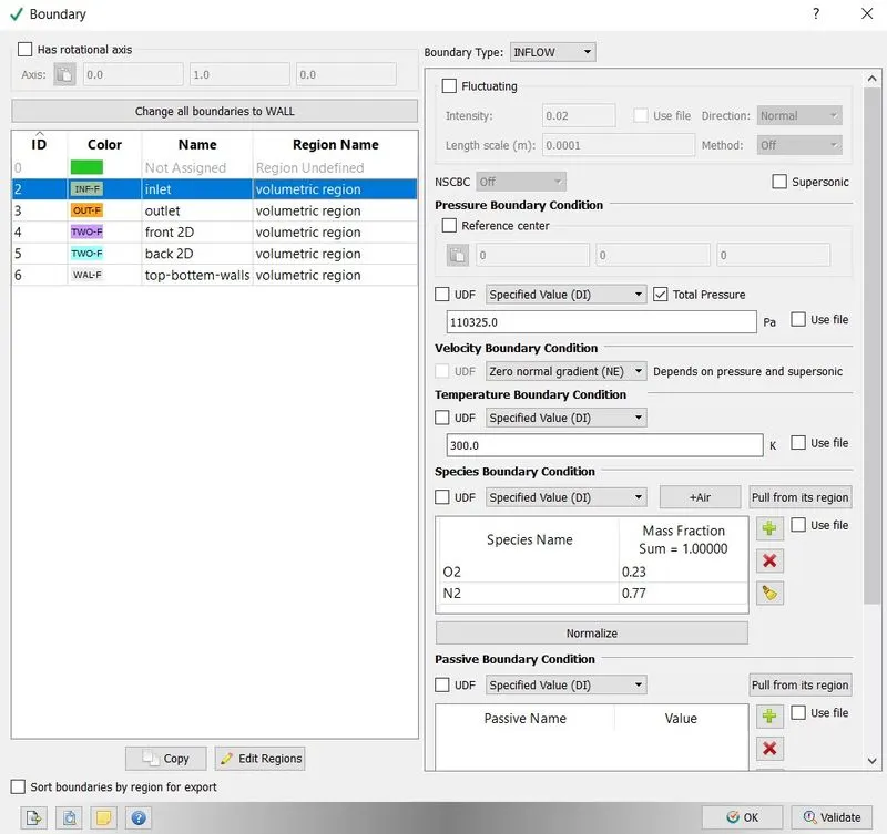
boundary-

• inlet- the inlet pressure(total pressure) i have taken is 110325 pascals.

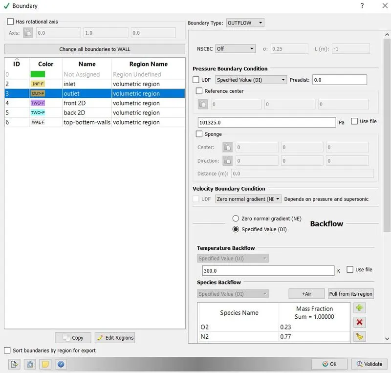
• outlet- the outlet pressure(static pressure) i have taken is 101325 pascals

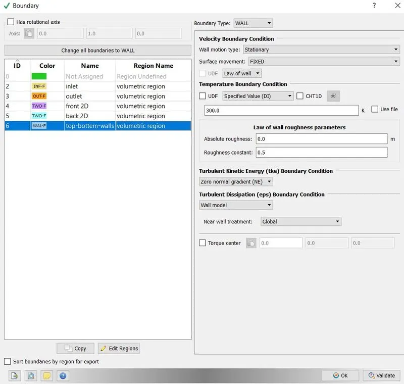
• top-bottem-wall - for the turbulent flows, we have to take law of wall.

• front 2D and back 2D-

physical models:

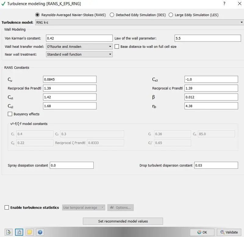
turbulence modelling-

grid control:

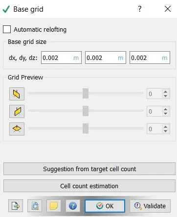
base grid-

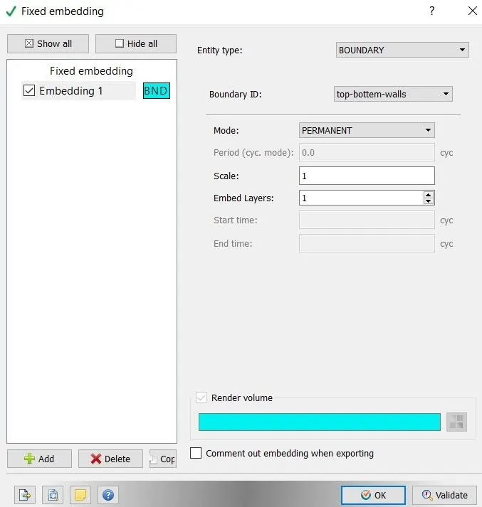
fixed embedding- i have enabled fixed embedding because to scale the cells at walls of the geometry. it means to to capture the turbulence in the turbulence boundary layer region, we have to provide cells with small size at the walls of the boundary.

output/post-processing:

post variable selection-

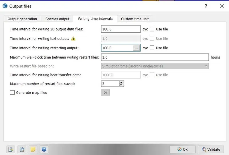
output-

solution:

now export all the input files in a folder. so from this we can see that converge is used to create the input files for the simulation. now insert the two application files from the converge folder to the folder where i have exported all the input files.

for the simulation i have used cygwin64 terminal. in cygwin termpinal open the folder where you have pasted all the input and application files.

now for the simulation write mpiexec.exe -n 4 converge.exe restricted and click enter. here 4 represents the number of processors used at a time.

post processing of results:

for this copy post convert application from converge folder to output folder which is generated in the input files folder. we are doing this because we are goingto convert all the output files into a vtk file which can be easily read by paraview software. toconvert the files we have to use post conver application as shown in the figure. there we can see the results that are obtained. now in cygwin open the output folder and write mpiexec.exe -n 4 post_convert.exe and click enter. now the below figure will appear

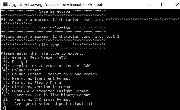
after naming the case and choosing 10, hit enter. now click yes for boundary output surface. now all the output files will appear and then write 'all' to convert all the output files. now select 'all' at cell variable selection menu. now all the files gets converted into paraview vtk files.

now open paraview. in paraview, open file and select case name .. vtm file which is present in the output files. finally we see the geometry in the paraview. now choose slice tool to select the axis along which all the primitive variables are same. as we know that, along z axis the primitive varibles are equal. so select axis and click apply.

• dx = dy = dz =2e-3 m

mesh -

velocity contour-

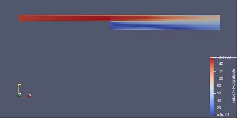
velocity vectors at recirculation zone-

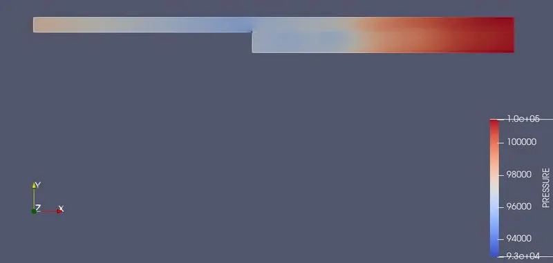
pressure contour-

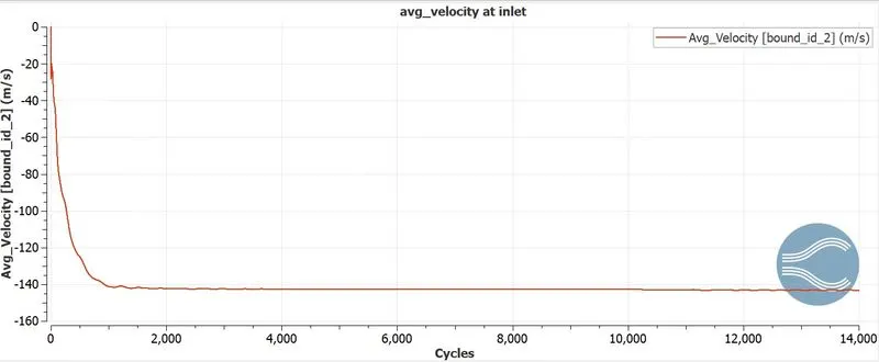
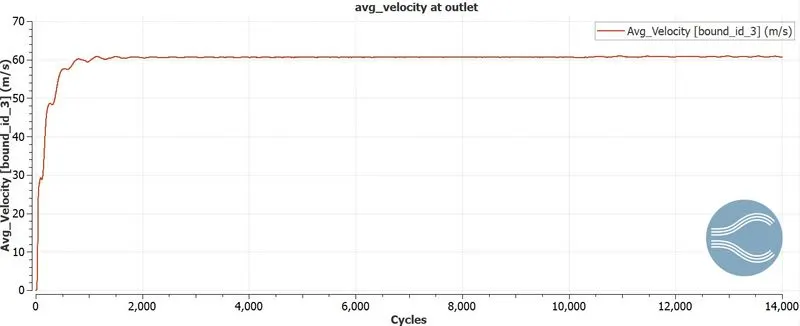
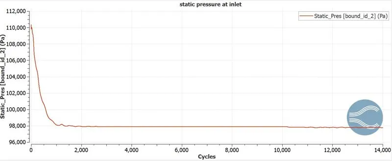
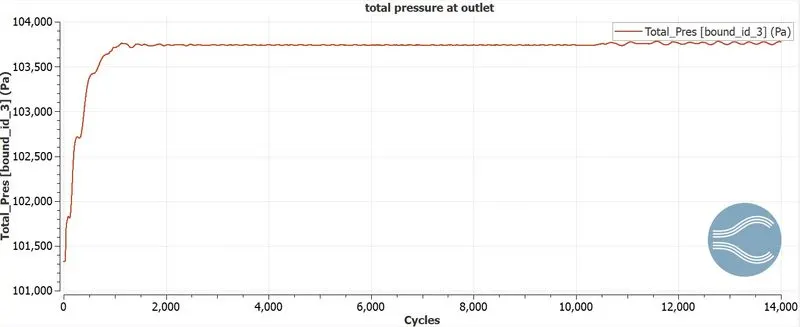
i have created the below plots in the converge.

velocity at inlet plot-

velocity at outlet plot-

static pressure at inlet-

total pressure at outlet-

mass flow rate at inlet-

mass flow rate at outlet-

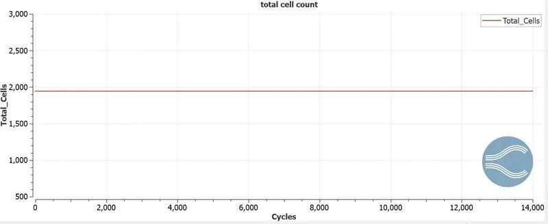
total cell count-

animation for above simulation-

• dx = dy = dz =1.5e-3 m

mesh-

velocity contour-

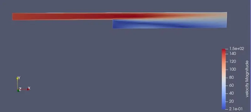
velocity vectors at recirculated zone-

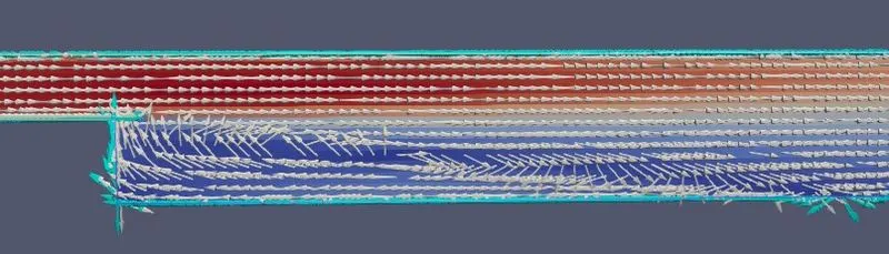
pressure contour-

velocity at inlet plot-

velocity at outlet plot-

static pressure at inlet plot-

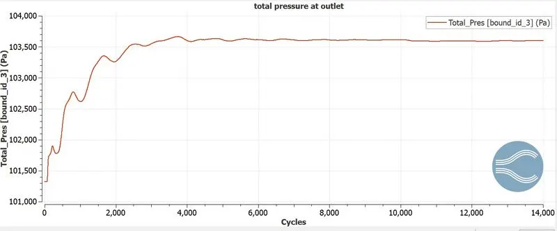
total pressure at outlet plot-

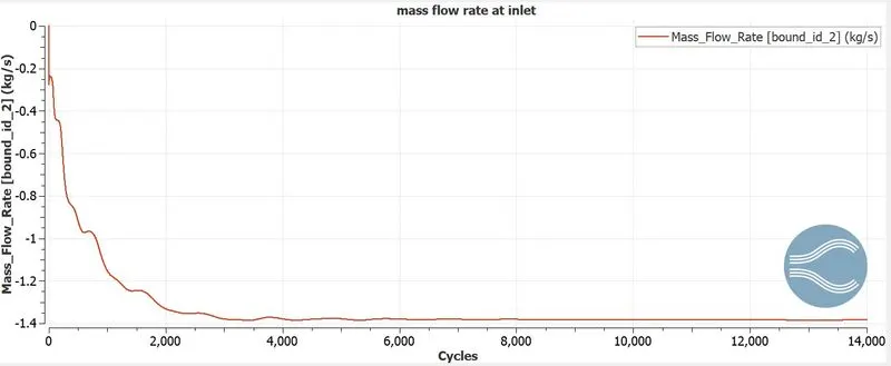
mass flow rate at inlet-

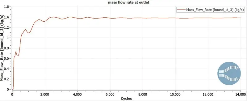
mass flow rate at outlet-

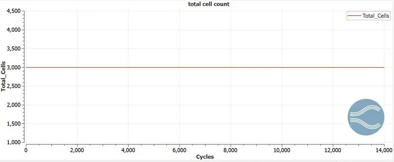
total cell count-

animation for above simulation-

• dx = dy = dz =1.0e-3 m

mesh-

velocity contour-

velocity vectors at recirculation region-

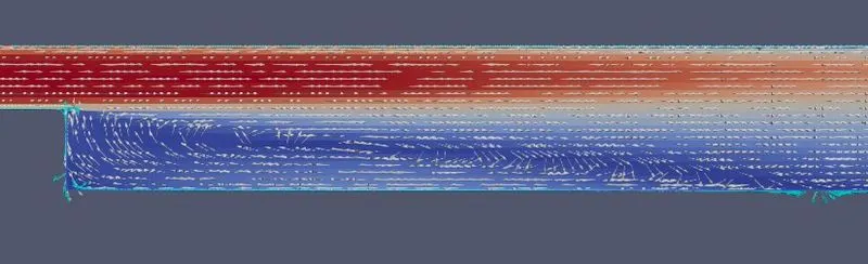
here the recirculation is generated during the flow. this occurs because as the fluid flow from smaller diameter pipe to larger diameter pipe, the fluid strike the larger diamter pipe at some distance from the facing step. so there will be a gap is generated between facing step to the fluid striking place. in the gap there will be less pressure as there is niw fluid is present . so the fluid gets back to that gap due to pressure difference. due to this recirculation gets occuers in the gap.

pressure contour-

velocity at inlet plot-

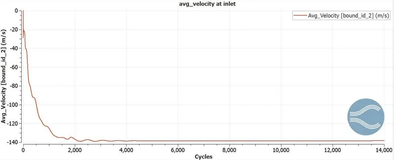
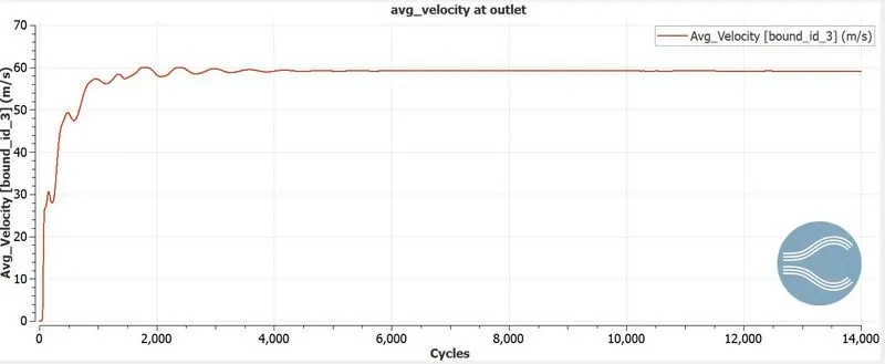
velocity at outlet plot-

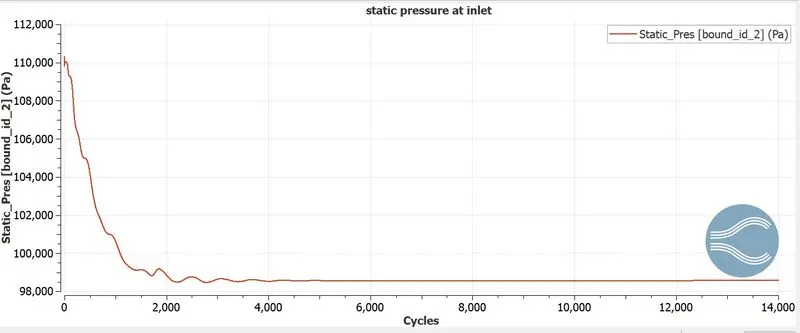
static pressure at inlet-

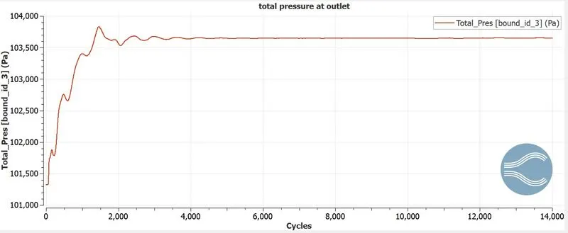
total pressure at outlet-

mass flow rate at inlet-

mass flow rate at outlet-

total cell count-

animation for above simulation-

conclusion:

• with decrease in cell size, the number of cells gets increased.
• with decrease in cell size. the time taken for simulation increases.
• with decrease in cell size, the simulation and the primitive variables are clearly visualized.