Week 6: Conjugate Heat Transfer Simulation
AIM:
conjugate heat transfer simulation on a pipe
objectives:
Grid dependence test-
- Start with an initial base grid
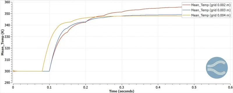
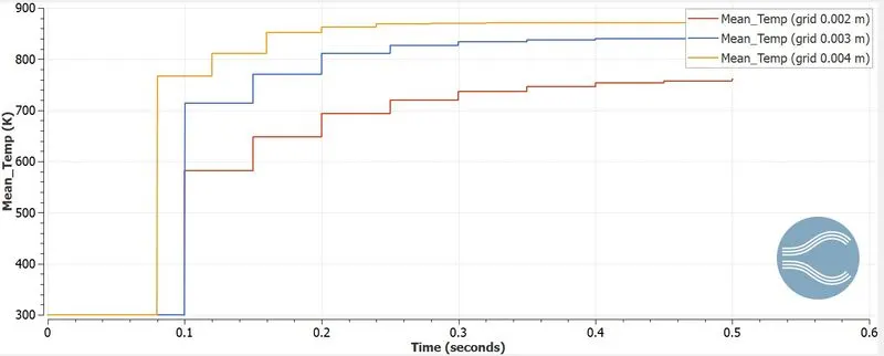
- Run grid dependence test on 3 grids and show that the outlet temperature converges to a particular value
Effect of supercycle stage interval-
- Set supercyle stage interval to 0.01,0.02 and 0.03
- For these three values, how does the total simulation time compare against the baseline configuration
theory:
Conjugate heat transfer:
Conjugate heat transfer corresponds with the combination of heat transfer in solids and heat transfer in fluids. In solids, conduction often dominates whereas in fluids, convection usually dominates. Conjugate heat transfer is observed in many situations. For example, heat sinks are optimized to combine heat transfer by conduction in the heat sink with the convection in the surrounding fluid. The temperature field and the heat flux are continuous at the fluid/solid interface. However, the temperature field can rapidly vary in a fluid in motion: close to the solid, the fluid temperature is close to the solid temperature, and far from the interface, the fluid temperature is close to the inlet or ambient fluid temperature. The distance where the fluid temperature varies from the solid temperature to the fluid bulk temperature is called the thermal boundary layer. The thermal boundary layer size and the momentum boundary layer relative size is reflected by the Prandtl number.
Prandtl number = `(C_p . mu)/K`
where `C_p` is heat capacity at constant pressure (SI unit: J/kg.K)
`mu`is the absolute visosity (SI unit: NS/m^2)
K is the thermal conductivity (SI unit: W/m.k)
for the Prandtl number to equal 1, thermal and momentum boundary layer thicknesses need to be the same. A thicker momentum layer would result in a Prandtl number larger than 1. Conversely, a Prandtl number smaller than 1 would indicate that the momentum boundary layer is thinner than the thermal boundary layer. The Prandtl number for air at atmospheric pressure and at 20°C is 0.7. That is because for air, the momentum and thermal boundary layer have similar size, while the momentum boundary layer is slightly thinner than the thermal boundary layer. higher the thermal boundary layer, there will br higher the heat transfer from fluid to solid.
geometry:
opem converge and create a cylinder with length 0.2m and radius 0.015m and click apply. now to add the thickmess to the cylinder give the redius of the outer cylinder is 0.02m and the click apply. now delete the triangles at the inlet and outlet as they are overlap with each other. now create the triangles between inner diameter and the outer diameter. now use repair tool and patch the inlets and outlets with triangles . finally check the normals whether they are positioned towords the inwords the cylinder domain.
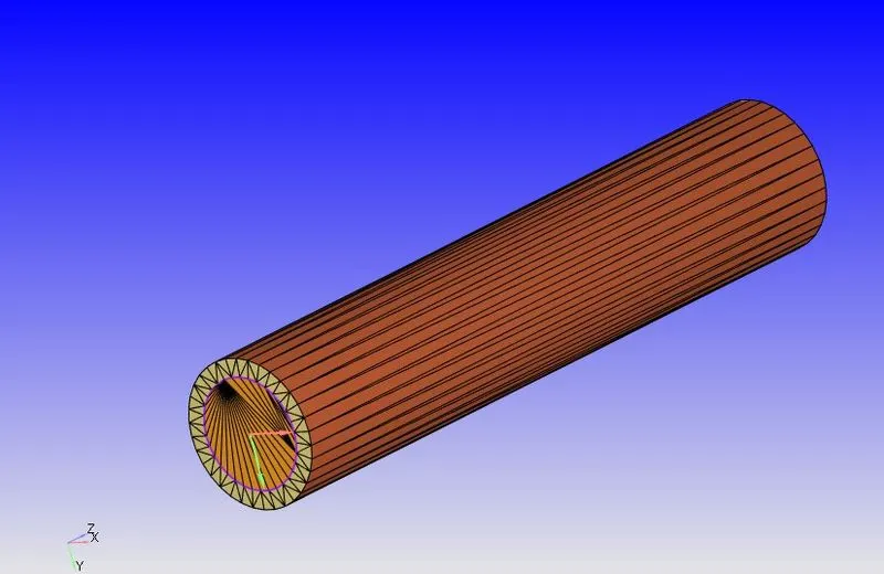
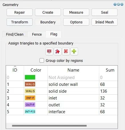
now name them using boundary flagging tool. name the outer surface of the cylinder as solid outer wall. name the thickness at inlet and outlet as solide side and then name the inlet and outlet. now select the inner surface of the cylinder and name it as interface.
now click on diagnosis and find the errors in creating the geometry. now we can see the error in non manifold edges because here on edge is shared by three triangles which are in inlet, solid side and the interface. here the simulation we are going to do is conjugate heat transfer so that we can neglet the error.
case setup:
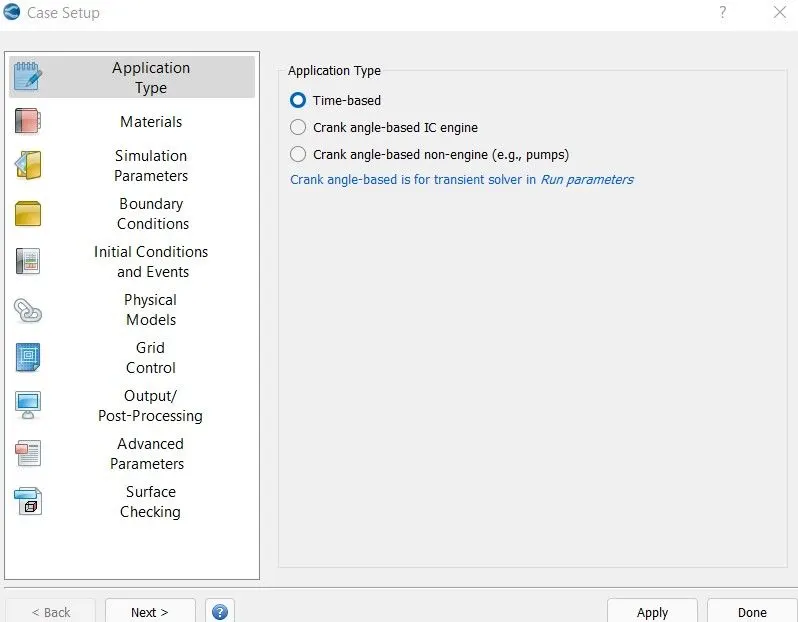
application type:
material:
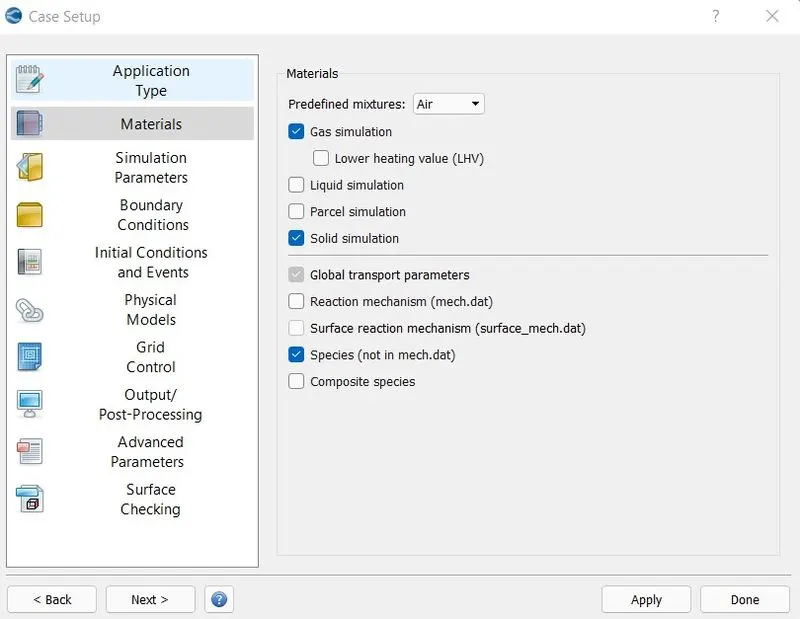
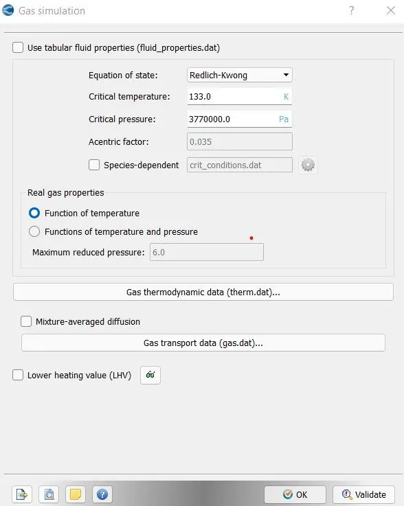
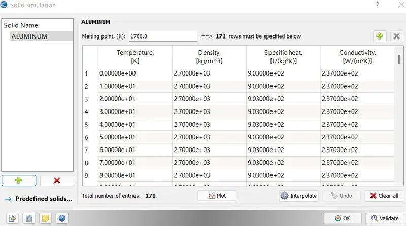
i have clicked on gas simulaion because here the the fluid(air ) moven in the cylinder through inet. i have clicked on solid simulation because here i am giving the heat to transfer from the solid part of the cylinder to fluid..
gas simulation-
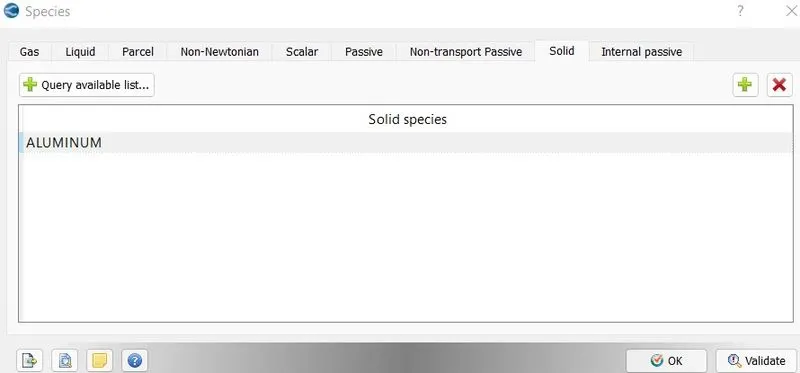
solid simulation- the material of cylinder i have taken is aluminium.
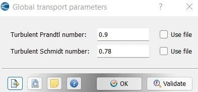
global transport parameters-
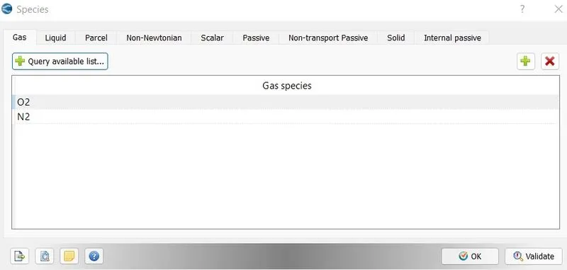
species-
simulation parameters:
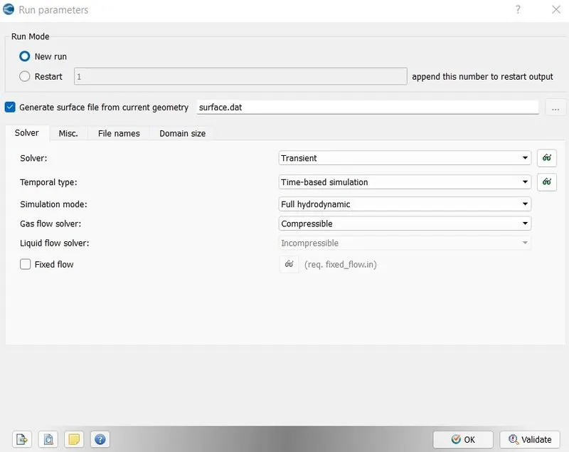
run parameters-
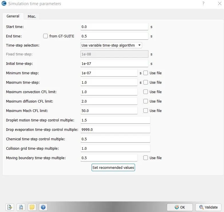
simulation time parameters-
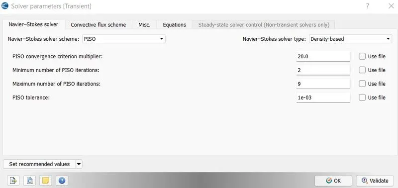
solver parameters-
initial conditions and events:
regions and initialization-
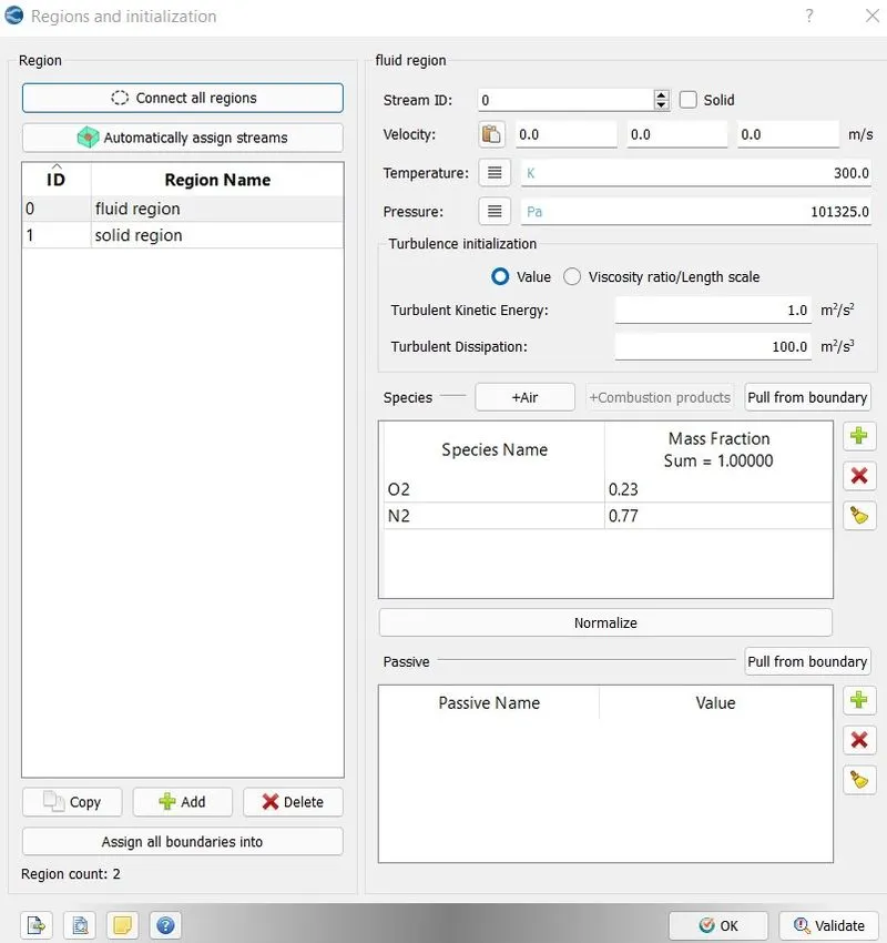
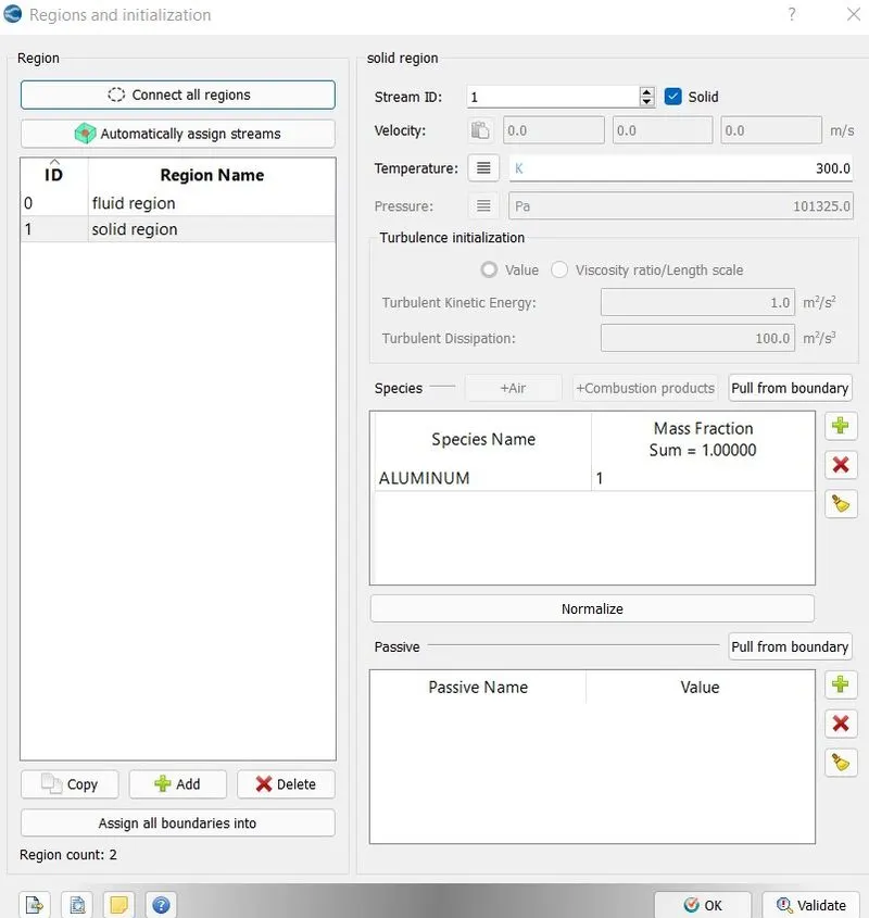
here i have created two regions because the simulation itself is a conjugate heat transfer simulation . i need the details of solid and fluid part that how the heat getting transferred through conduction and convection. while creating the solid region we have to give stream id. stream id-0 represents the fluid region and stream id-1 represents the static solid region and stream id >1 represents the moving solid region. here my solid is not moving, so i have taken the stram id as 1. the material in the solid region is aluminium. select that material in the solid region and select the air as amaterial in the fluid region.
boundary conditions:
boundary-
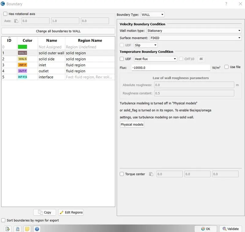
solid outer wall- here i have taken slip boundary condition . the heat flux that is transferring into the sold wall is 10000 w/m^2. i have taken the value as negative because the converge takes all the inputs as negative values.
solid side-
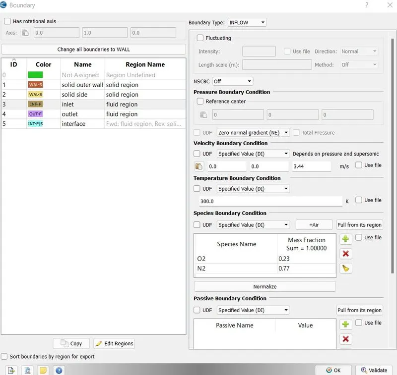
inlet-
the inlet reynolds number is 7000.
density of air = 1.225 kg/m^3
viscosity of air( at 15 degrees) = 1.81 × 10⁻⁵ kg/(m·s)
diameter of the pipe = 0.03 m
reynolds number = `(rho.v.d)/mu`
the velocity = 3.44 m/s, here the length of the pipe is along z axis. so i have take the velocity at z axis.
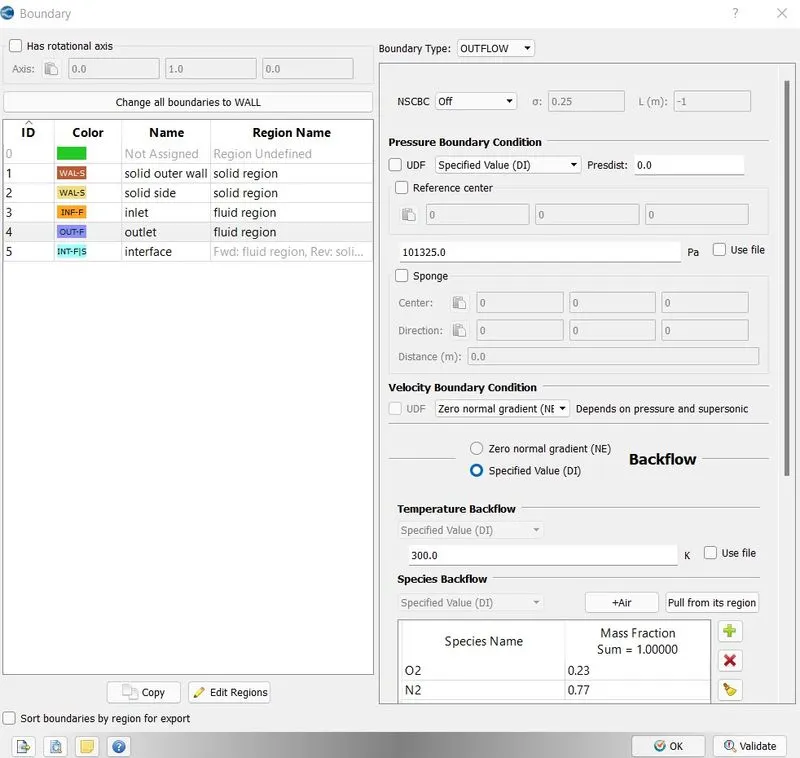
outlet-
interface- it is the one which connects the solid and flud region. so we can say that the interface is in both fluid and solid region. so in the converge the forward and reverse side are there. forward side represents the normals at the interface represents direction to the the region which we have to take. here the nromals are showing in to the fluid regin. so i have selected fluid region in the forward side.
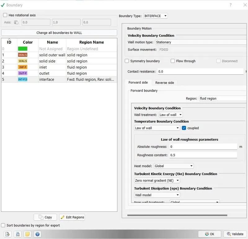
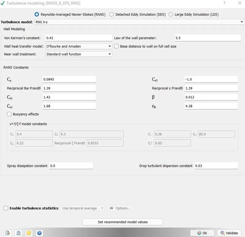
for the turbulent flows we have to take the law of wall boundary condition. below figure represnts the reverse side. here reverse side means the direction should ne along the outer surface of the cylinder. so i have taken slip boundary condition.
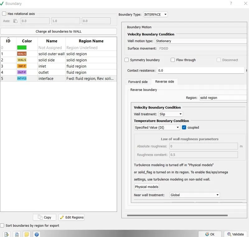
physical models:
turbulence modelling-
super cycle modelling-
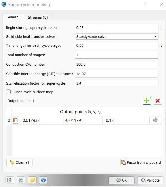
super cycling is the method used for the conjugate heat transfer problems. super cycling methos is the combination of both steady and transient state solver. in this problem, the heat has to transfer from cylinder to fluid. here our aim is to see the results at steady state position in both solids and fluids but fluids reaches to steady state position faster as compared to solids. so it will take more time to wait. to overcome this we ae going to use super cyling method. in this method i have mentioned the steady state solver to solid side. this method both the fluid and solid solvers run simulataneously, but the fluid solver remains paused after some time , but the solid solver still runs upto the solution reached to convergence. then again the fluid solver restarting the simulations. this process is till the simulation end time. here i have given that the fluid solver should remain pause for every seconds.
at the output section in the syper cycling, i have taken one point which is in between the interface and solid outer wall. we are going to see the means temperature of the solid at that point.
grid control:
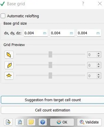
base grid-
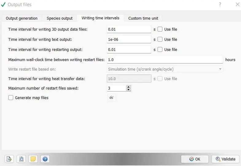
output-post processing:
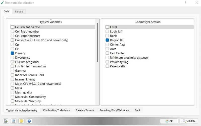
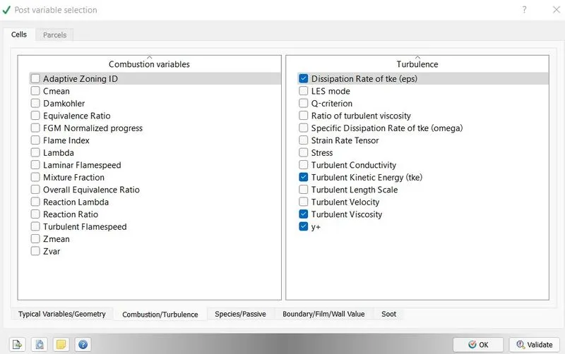
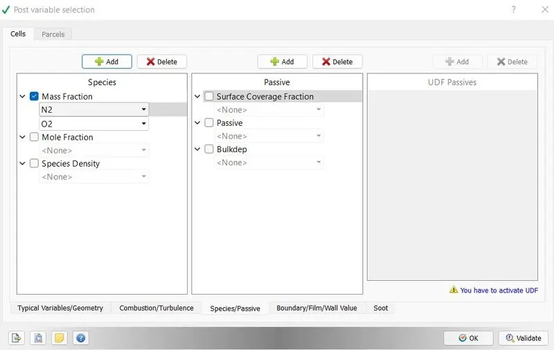
post variable selection-
output files:
solution:
now export all the input files in a folder. so from this we can see that converge is used to create the input files for the simulation. now insert the two application files from the converge folder to the folder where i have exported all the input files.

for the simulation i have used cygwin64 terminal. in cygwin termpinal open the folder where you have pasted all the input and application files.
now for the simulation write mpiexec.exe -n 4 converge.exe restricted and click enter. here 4 represents the number of processors used at a time.
post processing of results:

for this copy post convert application from converge folder to output folder which is generated in the input files folder. we are doing this because we are goingto convert all the output files into a vtk file which can be easily read by paraview software. toconvert the files we have to use post conver application as shown in the figure. there we can see the results that are obtained. now in cygwin open the output folder and write mpiexec.exe -n 4 post_convert.exe and click enter. now the below figure will appear
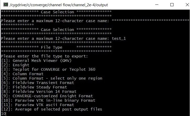
after naming the case and choosing 10, hit enter. now click yes for boundary output surface. now all the output files will appear and then write 'all' to convert all the output files. now select 'all' at cell variable selection menu. now all the files gets converted into varaview vtk files.
now open paraview. crate a slice along the z axis of the cylinder.
grid independence test:
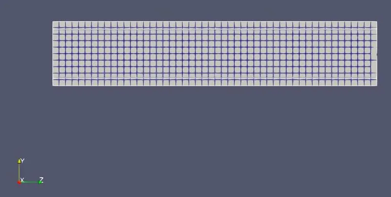
case 1- grid size 0.004 m
grid-
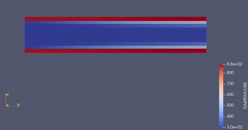
temperature contour-
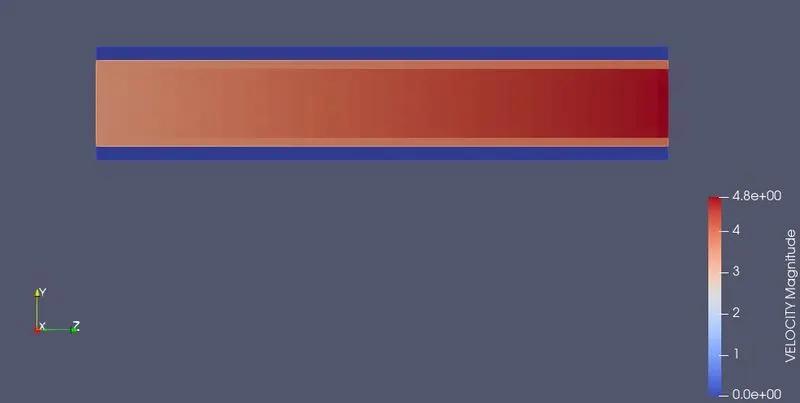
velocity contour-
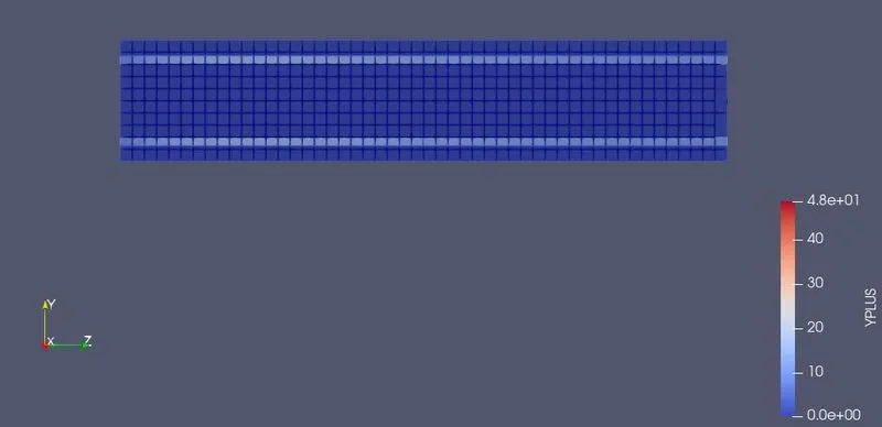
y+ contour-
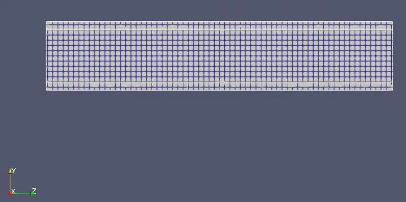
case 2-grid size 0.003m
grid-
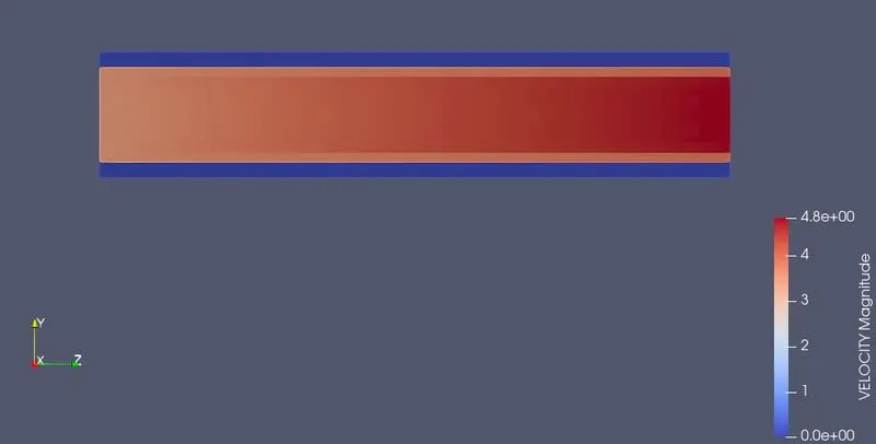
velocity contour-
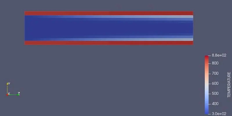
temperature contour-
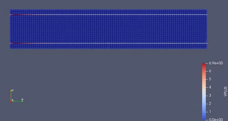
y+ contour -
case 3- grid size 0.002m
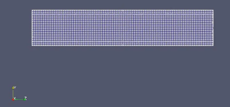
grid-
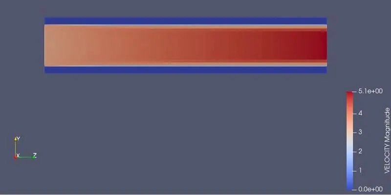
velocity contour-
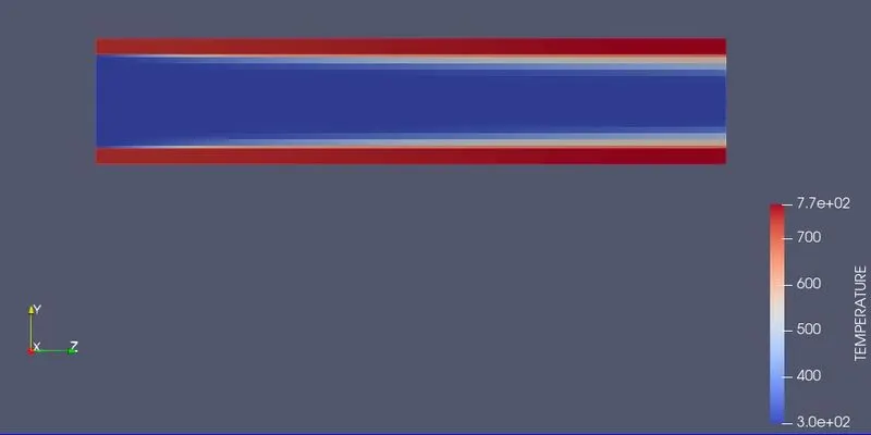
temperature contour-
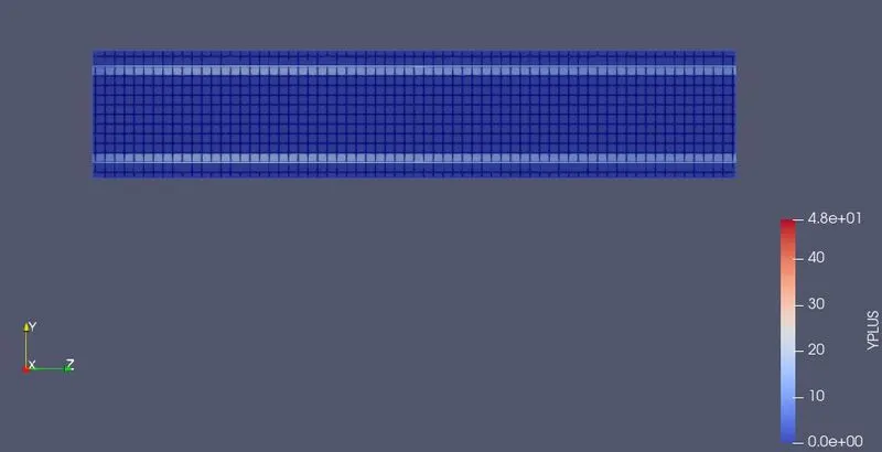
y+ contour-
velocity animation of aboe simulation-
temperature animation of above simulation-
mean temperature of fluid at different grid sizes-
mean temperature of solid at different grid sizes-
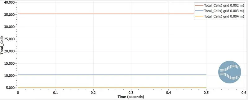
total cell count-
Effect of supercycle stage interval:
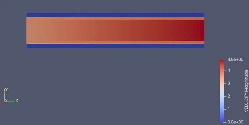
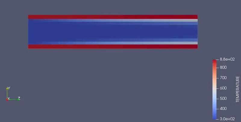
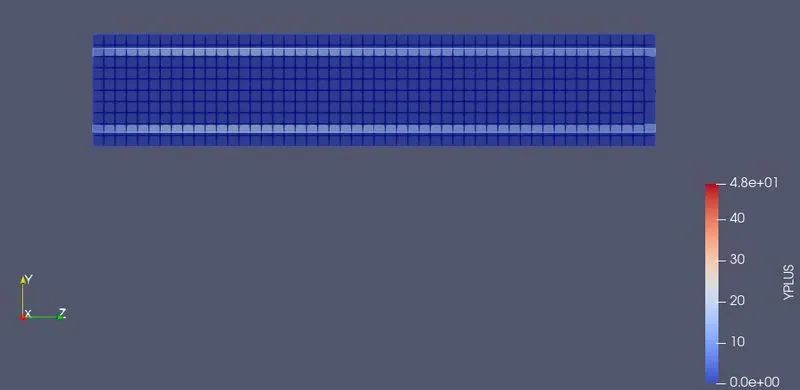
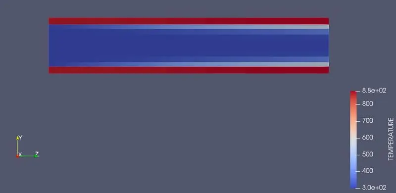
case 1 - with super cycle stage interval 0.01, grid size 0.004m
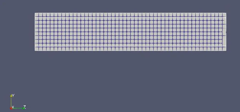
grid-
velocity contour-
temperature contour-
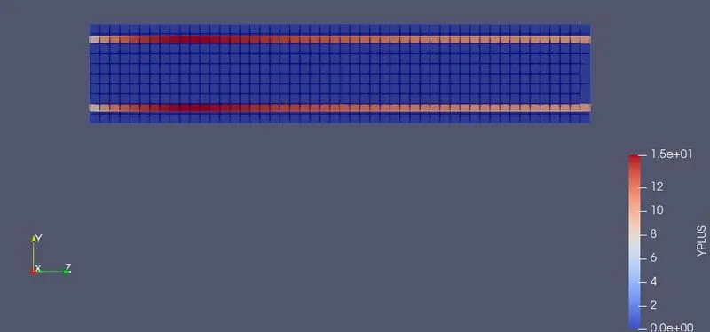
y+ contour-
velocity animation of above simulation-
temperature animation of above simulation-
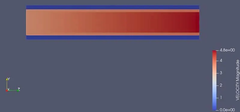
case 2 - with super cycling stage interval 0.02s, grid size 0.004m
grid-
velocity contour-
temperature contour-
y+ contour-
velocity animation of above simulation-
temperature animation of above simulation-
case 3- with super cycing stage interval 003 s, grid size 0.004 m
grid-
velocity contour-
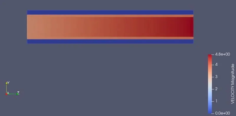
temperature contour-
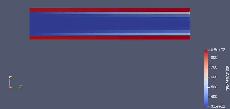
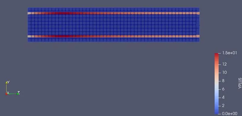
y+ contour-
velocity animation of above simulation-
temperature animation of above simulation-
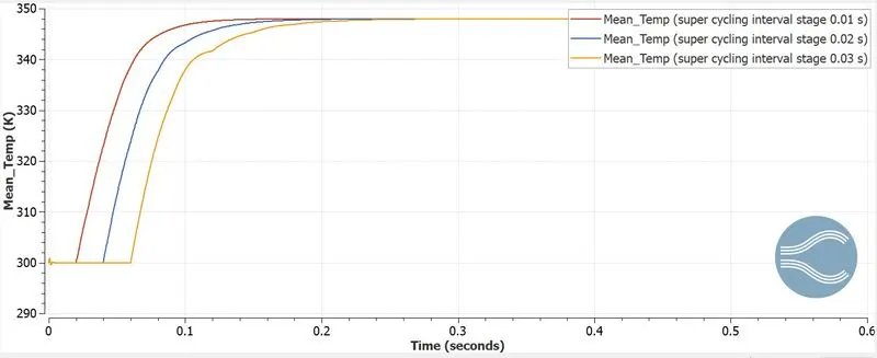
mean temperature of fluid at different super cycling intervals-
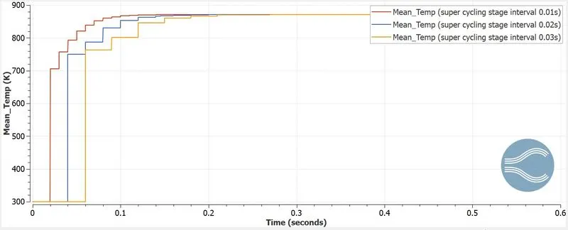
mean temperature of solid at different super cycling intervals-
| S.no | super cycling interval (seconds) | time taken for ruuning of simulation (seconds) |
| 1 | 0.01 | 288.58 |
| 2 | 0.02 | 357.82 |
| 3 | 0.03 | 395.49 |
conclusion:
- with decrease in size of the cell, we are clearly seeing the accurate mean temperatures in the fluid and solid.
- with decreasing of super cycling interval, the solutions reached to steady state faster
- with increase of super cycling interval, the time taken to run the simulation is increased.
- with change in grid size, the value of y+ also getting changes.