Week 6.2 - Setting up a model (Hanging Node)

Aim:

To perform thermal simulation of the given model i.e Hanging node.

Objectives:

1.Unpack the model into icepak

2.Generate mesh with Multi level settings to reduce No of nodes and elements (Done in assignment 2 week 5)

3.Perform thermal simulation of model in natural convection mode

4.Plot the contours of residuals and temperatures

Geometry:

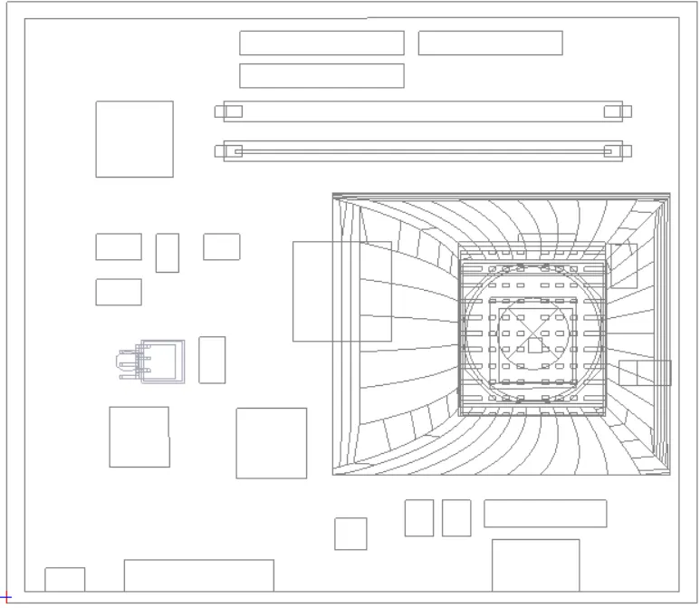
• The below picture the given CAD Model to generate the mesh using the multi-level parameters.
• The Geometry contains Fan, Capacitors, solid blocks, heat sink, and printed circuit boards, etc...

Meshing:

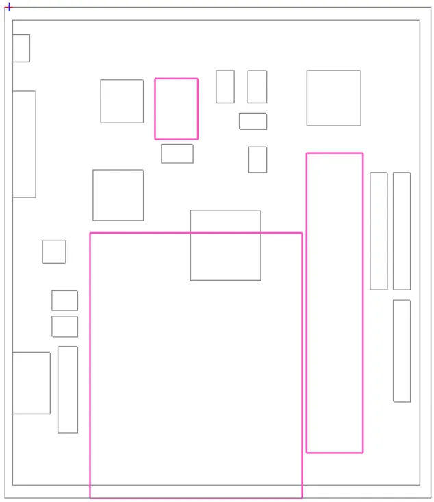
• For the first time, the mesh is generated for the Mesh assemblies separately. Which means a non-conformal mesh is performed.
• A non-conformal mesh, when there are a partial or zero matchings of nodes at the interface. This means that one, few, or every node on one side of the interface doesn’t have a match on the other side of the interface.

Multi-level meshing allows the user to refine the mesh locally in the areas where a higher mesh resolution is required to capture some geometrical features or gaps, while using a coarse Cartesian mesh in the rest of the model. The user can control the local mesh refinement using the "Max levels" option, which indicates the maximum number of levels that may be required to achieve the desired mesh refinement based on curvature/proximity. In the current model, multi-level meshing is allowed for the assemblies "sheetmetal_hs_assy.1" and "fan_guide.1". For both the assemblies, the "Max levels" option available in the "Multi-level settings" tab of the "Assemblies" window is set to 2. The objects "SheetMetal_HS" and "guide_sweep-0_1.1" are assigned "Max levels" equal to 2 in the "Multi-level meshing max levels" window for the assemblies "sheetmetal_hs_assy.1" and "fan_guide.1" respectively. For the assembly "sheetmetal_hs_assy.1", the maximum element size along each of the three coordinate directions (X, Y and Z) is set to 1 mm; the minimum gap along each of the three coordinate directions (X, Y and Z) is set to 0.06 mm. For the assembly "fan_guide.1", the maximum element size along each of the three coordinate directions (X, Y and Z) is set to 3 mm; the minimum gap along each of the three coordinate directions is set to 0.01 mm. The images attached below show the multi-level mesh settings applied for the assemblies "sheetmetal_hs_assy.1" and "fan_guide.1".

Multi level settings to reduce No of nodes and elements (Done in assignment 2 week 5)

The images attached below show the computational mesh plotted on three mutually perpendicular planes, each passing through the center of the cabinet.

1. X plane through center

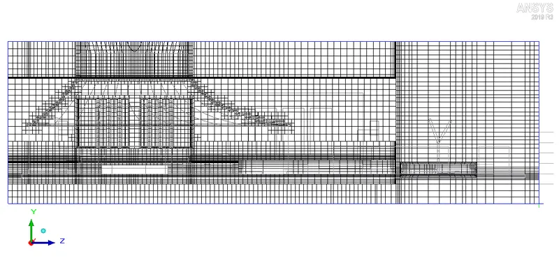
2. Y plane through center

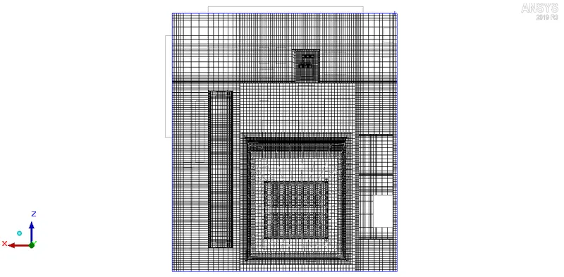
3. Z plane through center

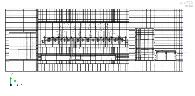
The images attached below show the surface mesh on the two CAD objects in the model:

1. SheetMetal_HS

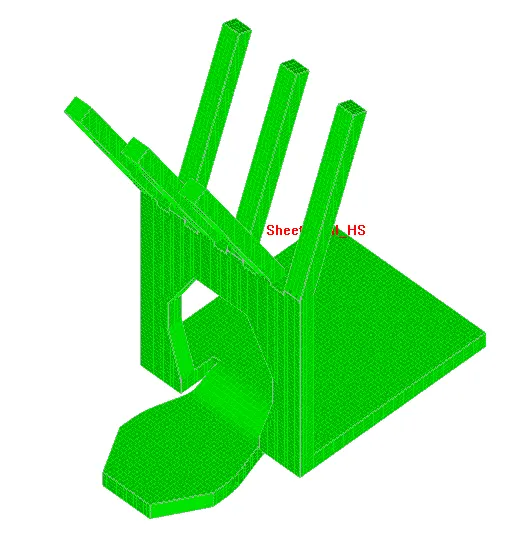
2. guide_sweep-0_1.1

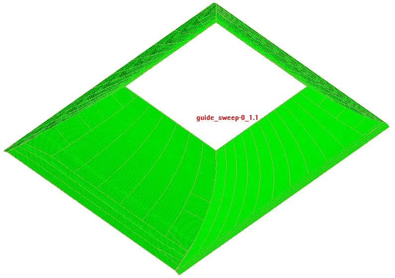
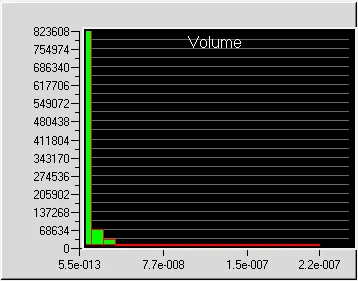
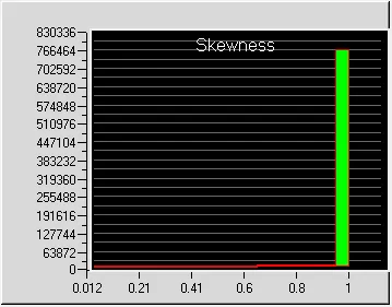
Visually the mesh appears to be fine. The images attached below show the histograms with the number of elements plotted along the X-axis and quality measures plotted along the Y-axis.

1. Face alignment

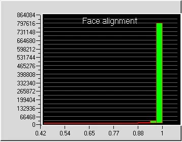
2. Volume

3. Skewness

Solver:

The three dimensional steady-state Navier-Stokes equations for the model are solved within the computational domain using the Fluent solver available in ANSYS Icepak. The following settings are applied to the solver:

1. Variables solved: Flow (velocity, pressure) and Temperature

2. Radiation: Off

3. Flow regime: Turbulent (Zero equation)

4. Time variation: Steady

5. Solution initialization

5.1. X velocity: 0

5.2. Y velocity: 0

5.3. Z velocity: 0

6. Number of iterations: 1000

7. Convergence criteria

7.1. Flow: 1e-7

7.2. Energy: 1e-10

7.3. Joule heating: 1e-7

8. Configuration: Parallel

9. Number of processors: 4

10. GPU computing: Enabled

11. Number of GPUs: 1

12. Precision: Double

Suitable heat generation values are assigned to various objects in the model and the fan is defined using the following settings:

1. Fan type: Internal

2. Flow direction: Normal (Negative)

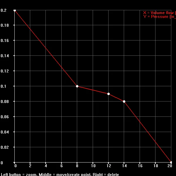
3. Flow type: Non-linear. The image attached below shows the non-linear performance curve of the fan.

4. RPM: 4000 rpm

Results:

In the current section, the simulation results are discussed.

Residuals:

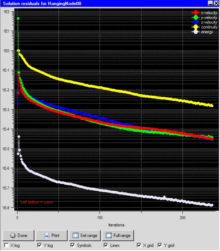
The residuals for the following equations are plotted against the number of iterations:

i. Continuity equation

ii. X-momentum equation

iii. Y-momentum equation

iv. Y-momentum equation

v. Z-momentum equation

vi. Energy equation

The image attached below shows the residuals plotted against the number of iterations.

Monitor plots:

Temperature and velocity monitor points are set up at various key locations within the computational domain. Apart from providing information about the solution variables (such as velocity, temperature, pressure etc.) at important locations within the computational domain, the monitor plots also help the user to determine if the solution has reached a steady state. The following five monitor points are created within the computational domain:

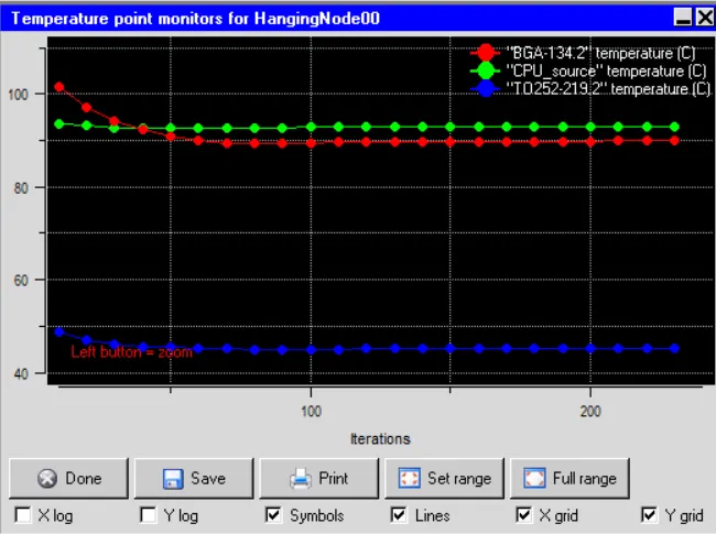
The plot shows that temperature values at the monitor points defined on the three objects, BGA-134.2, CPU_source and TO252-219.2, don't change appreciably beyond 200 iterations. This indicates that the energy equation has already converged, which is also shown by the small residual of the energy equation. According to the plot, the following steady-state temperature values are predicted by the monitor points defined in the model:

i. BGA-134.2: 95.98 °C

ii. CPU_source: 92.22 °C

iii. TO252-219.2: 44.45 °C

Velocity monitor plot:

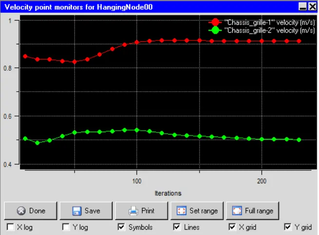
The plot shows that the velocity values at the monitor points defined on the two objects, Chassis_grille-1 and Chassis_grille-2, This indicates that the continuity and momentum equations have converged about 200 iterations. According to the plot, the following steady-state velocity values are predicted by the monitor points defined in the model.

i. Chassis_grille-1: 0.931 m/s

ii. Chassis_grille-2: 0.512 m/s

Temperature contours:

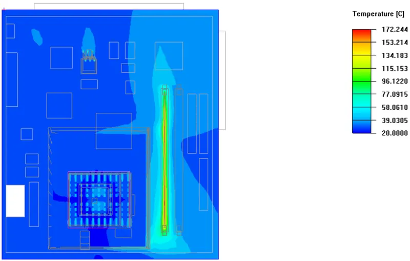
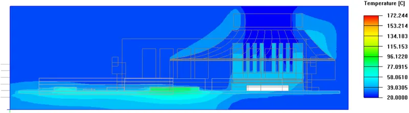
The steady-state temperature contours are plotted on two mutually perpendicular planes, each passing through the center of the cabinet, as shown in the images attached below.

Y-plane through center:

X-plane through center:

Z-plane through center:

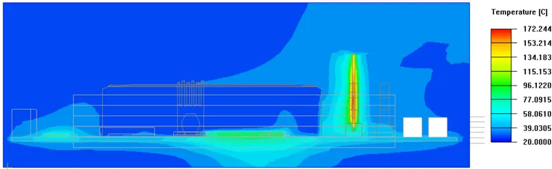
The contours show that the air inside the enclosure assembly is at a lower temperature than any other object. As it interacts with the hotter objects in the model, due to heat transfer from them, its temperature increases. As a result the air leaving the assembly is hotter than the air entering it. According to the plots the maximum temperature within the computational domain is 172°C

Velocity contours:

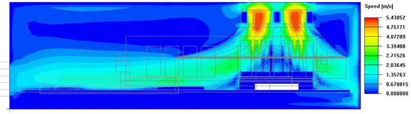
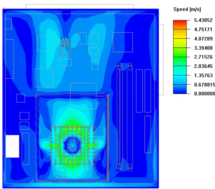
The steady-state velocity contours are plotted separately on two mutually perpendicular planes, each passing through the center of the cabinet as shown in the images attached below.

X-plane through center:

Y-plane through center:

Z-plane through center:

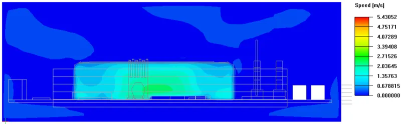
The contour plots show that the air velocity is highest as it moves through the fan. After passing through the fan, the air flows over different objects in the model (such as heat-sink, BGA etc.) which affect the flow field. Finally the air leaves the assembly through the two grilles. According to the contour plots, the maximum velocity within the computational domain is 5.43 m/s.

Velocity vectors:

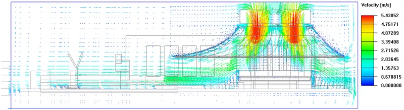
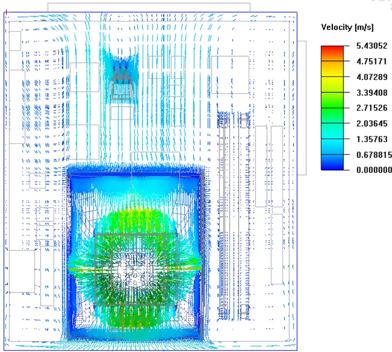
The steady-state velocity vectors are plotted on two mutually perpendicular planes, each passing through the center of the cabinet, as shown in the images attached below.

X-plane through center:

Y-plane through center:

Z-plane through center:

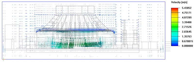
The vector plots show the velocity vectors for air at 5000 points distributed uniformly throughout the two planes (X-plane and Y-plane) passing through the center of the cabinet. The vectors are colored by the velocity magnitude. It is evident from the vectors that air achieves maximum velocity as it passes through the fan. The velocity vectors are also able to capture the recirculation zones established on the two planes (X-plane and Y-plane).

Object face temperature contours:

The steady-state temperature contours are plotted on the faces of all the objects that are located within the cabinet, as shown in the image attached below.

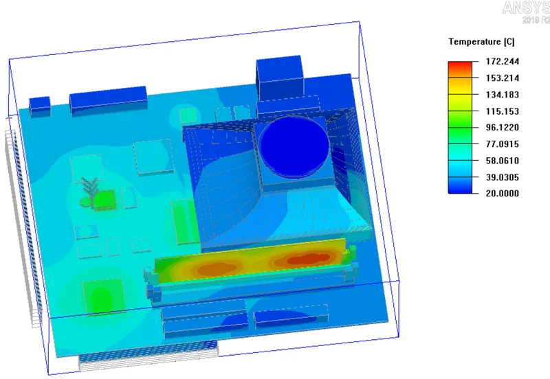
The contours show that the objects in the model that are assigned a power generation, attain higher temperatures at steady-state. Additionally the objects located near these power generating objects also attain relatively higher temperatures due to conduction heat transfer from them (power generating objects). According to the contours the maximum temperature attained by the objects within the cabinet is 172°C.