Week 5.1 - Mid term project - Solving the steady and unsteady 2D heat conduction problem
AIM: To solve 2D Heat conduction equation for steady and transient state using iterative methods such as jacobi, gauss seidel and successive over relaxation
Here we use 3 methods named
- Jacobi: In this we assume initial values at all nodes to calculate the new values,which we will update once we find all the nodes values and this continues untill we arrive with an converge solution.
- Gauss seidel: In this we assume the values obtained in jacobi iteration for the next equation.
- Successive over relaxtion(SOR):This an updated version of previous two.
For Steady State Flow:
clear all
close all
clc
%initial conditions
% grid points in x and y direction
nx=30;
ny=30;
%length of domain
L=1;
x=linspace(0,L,nx);
y=linspace(0,L,ny);
error=9e9;
tol=1e-4;
%Boundary conditions
T_L=400;
T_T=600;
T_R=800;
T_B=900;
T=ones(nx,ny);
% Temperature @ boundary
T(2:ny-1,1)=T_L;
T(2:ny-1,nx)=T_R;
T(1,2:nx-1)=T_T;
T(nx,2:ny-1)=T_B;
%temperature @ corner by average value temp
T(1,1)=(T_T+T_L)/2;
T(nx,ny)=(T_R+T_B)/2;
T(1,ny)=(T_T+T_R)/2;
T(nx,1)=(T_L+T_B)/2;
% factors considered
[X,Y]=meshgrid(x,y);
 Told=T;
 %2D steady state heat conduction equation
 for iterative_solver=1
 tic;
if iterative_solver==1
 jacobi_iter=1;
 while(error>tol)
     for i=2:nx-1
         for j=2:ny-1
           T(i,j)=0.25*(Told(i-1,j)+Told(i+1,j)+Told(i,j-1)+Told(i,j+1));
         end
     end
     error=max(max(abs(Told-T)));
     Told=T;
     jacobi_iter=jacobi_iter+1;
 end
 end
 F=toc;

 figure(1)
 [a,b]=contourf(X,Y,T);
 clabel(a,b)
 colormap(jet)
 xlabel('X axis');
 ylabel('Y axis');
 colorbar
 hold on
 title_text=sprintf('jacobi no of iteration=%d,Total time F=%fs',jacobi_iter,F);
 title(title_text)
 fprintf('Number of iteration done are =%d \n',jacobi_iter);
 end

%GS Iter
nx=30;
ny=30;
%length of domain
L=1;
x=linspace(0,L,nx);
y=linspace(0,L,ny);
error=9e9;
 %for SOR
tol=1e-4;
%Boundary conditions
T_L=400;
T_T=600;
T_R=800;
T_B=900;
T=ones(nx,ny);
% Temperature @ boundary
T(2:ny-1,1)=T_L;
T(2:ny-1,nx)=T_R;
T(1,2:nx-1)=T_T;
T(nx,2:ny-1)=T_B;
%temperature @ corner by average value temp
T(1,1)=(T_T+T_L)/2;
T(nx,ny)=(T_R+T_B)/2;
T(1,ny)=(T_T+T_R)/2;
T(nx,1)=(T_L+T_B)/2;
[X,Y]=meshgrid(x,y);
Told=T;
for iterative_solver=2
tic;
if iterative_solver==2
gs_iter=2;
while(error>tol)
    for i=2:nx-1
        for j=2:ny-1
            T(i,j)=0.25*(T(i-1,j)+Told(i+1,j)+T(i,j-1)++Told(i,j+1));
        end
    end
 error =max(max(abs(Told-T)));
 Told=T;
 gs_iter=gs_iter+1;
end
end
F=toc;
figure(2)
contourf(X,Y,T);
[a,b]=contourf(X,Y,T);
clabel(a,b);
colormap(jet)
xlabel('X axis')
ylabel('Y axis')
hold on
colorbar
title_text=sprintf('Guass no of iteration=%d,Total time F=%fs',gs_iter,F);
title(title_text)
fprintf('Number of iteration done are =%d\n',gs_iter);
end

%SOR Iter
%initial conditions
% grid points in x and y direction
nx=30;
ny=30;
%length of domain
L=1;
x=linspace(0,L,nx);
y=linspace(0,L,ny);
error=9e9;
%for SOR
alpha=1.8;
tol=1e-4;
%Boundary conditions
T_L=400;
T_T=600;
T_R=800;
T_B=900;
T=ones(nx,ny);
% Temperature @ boundary
T(2:ny-1,1)=T_L;
T(2:ny-1,nx)=T_R;
T(1,2:nx-1)=T_T;
T(nx,2:ny-1)=T_B;
%temperature @ corner by average value temp
T(1,1)=(T_T+T_L)/2;
T(nx,ny)=(T_R+T_B)/2;
T(1,ny)=(T_T+T_R)/2;
T(nx,1)=(T_L+T_B)/2;

[X,Y]=meshgrid(x,y);
Told=T;
for iterative_solver=3
tic;
if iterative_solver==3
sor_iter=1;
while(error>tol)
    for i=2:nx-1
        for j=2:ny-1
            T(i,j)=((1-alpha)*Told(i,j)+(alpha*0.25*(T(i,j-1)+Told(i,j+1)+T(i-1,j)+Told(i+1,j))));
        end
    end

   error=max(max(abs(Told-T)));
   Told=T;
   sor_iter=sor_iter+1;
end
end
F=toc;
figure(3)
contourf(X,Y,T);
[a,b]=contourf(X,Y,T);
clabel(a,b);
xlabel('X axis')
ylabel('Y axis')
hold on
colorbar
colormap(jet)
title_text= sprintf('SOR no of iterations=%d,Total time F=%fs',sor_iter,F);
title(title_text)
fprintf('No of iteration in SOR=%d \n',sor_iter);
end
Steady Program output:
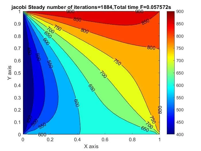
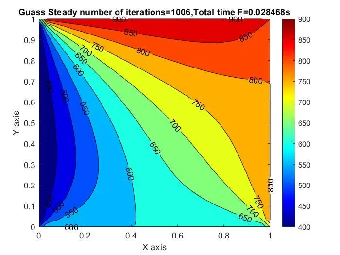
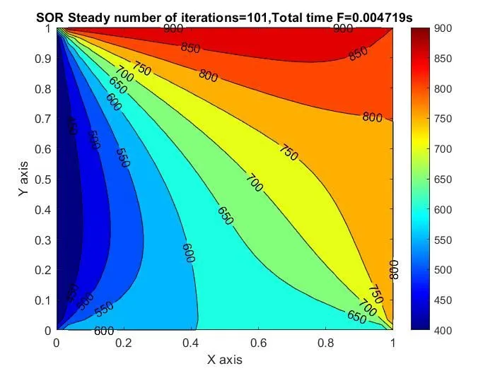
From the above results we can conclude that SOR is the faster method, the number of iteration and stability of the solution depends upon the relaxation factor
FOR UNSTEADY STATE FLOW:
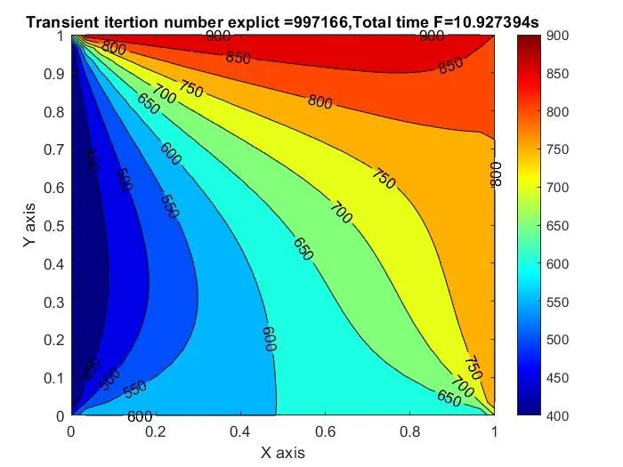
Explicit Method:The temperature at next level is calculated by means of surrounding temperature values and increasing time steps i.e dt shall result in oscillation of result solution diverges from original result.
2D Transient equation solved explicitly:
close all
clear all
clc
%no of grid points
nx=30;
ny=30;
L=1;%length of domain
x=linspace(0,L,nx);
y=linspace(0,L,ny);
dx=x(2)-x(1);
dy=y(2)-y(1);
error=9e9;
tol=1e-4;
dt=0.01;
%Thermal diffusivity for steel
alpha=1.88e-5;
%B.Cs
T_L=400;
T_T=600;
T_R=800;
T_B=900;
T=ones(nx,ny);
T(2:ny-1,1)=T_L;
T(2:ny-1,nx)=T_R;
T(1,2:nx-1)=T_T;
T(nx,2:ny-1)=T_B;
%Average temperature
T(1,1)=(T_T+T_L)/2;
T(nx,ny)=(T_R+T_B)/2;
T(1,nx)=(T_T+T_R)/2;
T(nx,1)=(T_L+T_B)/2;
%K constants
k1=(alpha*dt)/(dx^2);
k2=(alpha*dt)/(dy^2);
[X,Y]=meshgrid(x,y);
Told=T;
%2D transient state heat conduction for explicit
iterative_solver=1;
tic;
if iterative_solver==1
solver_counter=1;
while(error>tol)
    for i=2:nx-1
        for j=2:ny-1
            term1=Told(i,j);
            term2=k1*(Told(i+1,j)-2*Told(i,j)+Told(i-1,j));
            term3=k2*(Told(i,j+1)-2*Told(i,j)+Told(i,j-1));
            T(i,j)=term1+term2+term3;
        end
    end
    error= max(max(abs(Told-T)));
    Told=T;
    solver_counter=solver_counter+1;
end

F=toc;
%plot
figure(1)
[a,b]=contourf(X,Y,T);
clabel(a,b)
colormap(jet)
colorbar
title_text=sprintf('Transient itertion number explict =%d,Total time F=%fs',solver_counter,F);
title(title_text)
xlabel('X axis')
ylabel('Y axis')
fprintf('No of iterations in transient(explict)=%d\n',solver_counter)
end
Transient flow (explicit) output:
Transient flow (Implicit-Jacobi,Gauss siedel and SOR):
clear all
close all
clc
% no of grid points
nx=30;
ny=30;
L=1;
x=linspace(0,L,nx);
y=linspace(0,L,ny);
dx=x(2)-x(1);
dy=y(2)-y(1);
error=9e9;
tol=1e-4;
dt=2000;
% thermal diffusivity for steel
alpha=1.88e-5;
%B.Cs
T_L=400;
T_T=600;
T_R=800;
T_B=900;
T=ones(nx,ny);
T(2:ny-1,1)=T_L;
T(2:ny-1,nx)=T_R;
T(1,2:nx-1)=T_T;
T(nx,2:ny-1)=T_B;
%Average temperature
T(1,1)=(T_T+T_L)/2;
T(nx,ny)=(T_R+T_B)/2;
T(1,nx)=(T_T+T_R)/2;
T(nx,1)=(T_L+T_B)/2;
% values for constants K
k1=(alpha*dt)/(dx^2);
k2=(alpha*dt)/(dy^2);
[X,Y]=meshgrid(x,y);
Told=T;
T_Prev_dt=Told;
%2D Transient state heat conduction for implicit
iterative_solver=1:3;
%jacobi iteration
term1=(1+2*k1+2*k2)^(-1);
term2=k1*term1;
term3=k2*term1;
for iterative_solver=1
tic;
if iterative_solver==1
    jacobi_iter=1;
   while(error>tol)
     for i=2:nx-1
         for j=2:ny-1
             H=(Told(i-1,j)+Told(i+1,j));
             V=(Told(i,j-1)+Told(i,j+1));
             T(i,j)=term1*T_Prev_dt(i,j)+term2*H+term3*V;
         end
     end
     error=max(max(abs(Told-T)));
     Told=T;
     jacobi_iter=jacobi_iter+1;
   end
end
F=toc;
 figure(1)
 [a,b]=contourf(X,Y,T);
 clabel(a,b)
 colormap(jet)
 xlabel('X axis');
 ylabel('Y axis');
 colorbar
 hold on
 title_text=sprintf('jacobi transient(Implicit) number of iterations=%d,Total time F=%fs',jacobi_iter,F);
 title(title_text)
 fprintf('Number of iteration done are =%d \n',jacobi_iter);
end

% no of grid points
nx=30;
ny=30;
L=1;
x=linspace(0,L,nx);
y=linspace(0,L,ny);
dx=x(2)-x(1);
dy=y(2)-y(1);
error=9e9;
tol=1e-4;
dt=2000;
% thermal diffusivity for steel
alpha=1.88e-5;
%B.Cs
T_L=400;
T_T=600;
T_R=800;
T_B=900;
T=ones(nx,ny);
T(2:ny-1,1)=T_L;
T(2:ny-1,nx)=T_R;
T(1,2:nx-1)=T_T;
T(nx,2:ny-1)=T_B;
%Average temperature
T(1,1)=(T_T+T_L)/2;
T(nx,ny)=(T_R+T_B)/2;
T(1,nx)=(T_T+T_R)/2;
T(nx,1)=(T_L+T_B)/2;
% values for constants K
k1=(alpha*dt)/(dx^2);
k2=(alpha*dt)/(dy^2);
[X,Y]=meshgrid(x,y);
Told=T;
T_Prev_dt=Told;
term1=(1+2*k1+2*k2)^(-1);
term2=k1*term1;
term3=k2*term1;
for iterative_solver=2
tic;
if iterative_solver==2
    gs_iter=1;
    while(error>tol)
         for i=2:nx-1
            for j=2:ny-1
               H=(T(i-1,j)+Told(i+1,j));
               V=(T(i,j-1)+Told(i,j+1));
               T(i,j)=term1*T_Prev_dt(i,j)+term2*H+term3*V;
            end
         end
         error =max(max(abs(Told-T)));
         Told=T;
         gs_iter=gs_iter+1;
    end
end
F=toc;
figure(2)
contourf(X,Y,T);
[a,b]=contourf(X,Y,T);
clabel(a,b);
colormap(jet)
xlabel('X axis')
ylabel('Y axis')
hold on
colorbar
title_text=sprintf('Guass transient(Implicit) number of iterations=%d,Total time F=%fs',gs_iter,F);
title(title_text)
fprintf('Number of iteration done are =%d\n',gs_iter);
end

% no of grid points
nx=30;
ny=30;
L=1;
x=linspace(0,L,nx);
y=linspace(0,L,ny);
dx=x(2)-x(1);
dy=y(2)-y(1);
error=9e9;
tol=1e-4;
dt=2000;
% thermal diffusivity for steel
alpha=1.88e-5;
% thermal diffusivity for SOR
alpha1=1.8;
%B.Cs
T_L=400;
T_T=600;
T_R=800;
T_B=900;
T=ones(nx,ny);
T(2:ny-1,1)=T_L;
T(2:ny-1,nx)=T_R;
T(1,2:nx-1)=T_T;
T(nx,2:ny-1)=T_B;
%Average temperature
T(1,1)=(T_T+T_L)/2;
T(nx,ny)=(T_R+T_B)/2;
T(1,nx)=(T_T+T_R)/2;
T(nx,1)=(T_L+T_B)/2;
% values for constants K
k1=(alpha*dt)/(dx^2);
k2=(alpha*dt)/(dy^2);
[X,Y]=meshgrid(x,y);
Told=T;
T_Prev_dt=Told;

term1=(1+2*k1+2*k2)^(-1);
term2=k1*term1;
term3=k2*term1;
for iterative_solver=3
    tic;
    if iterative_solver==3
        sor_iter=1;
        while(error>tol)
            for i=2:nx-1
                for j=2:ny-1
                    H=(alpha1*T(i-1,j)+(1-alpha1)*Told(i-1,j)+Told(i+1,j));
                    V=(alpha1*T(i,j-1)+(1-alpha1)*Told(i,j-1)+Told(i,j+1));
                    T(i,j)=term1*T_Prev_dt(i,j)+(term2*H+term3*V);
                end
            end
            error=max(max(abs(Told-T)));
            Told=T;
            sor_iter=sor_iter+1;
        end
    end
F=toc;
%Plot
figure(3)
contourf(X,Y,T);
[a,b]=contourf(X,Y,T);
clabel(a,b);
xlabel('X axis')
ylabel('Y axis')
hold on
colorbar
colormap(jet)
title_text= sprintf('SOR transient(Implicit) number of iterations=%d,Total time F=%fs',sor_iter,F);
title(title_text)
fprintf('No of iteration in SOR=%d \n',sor_iter);
end
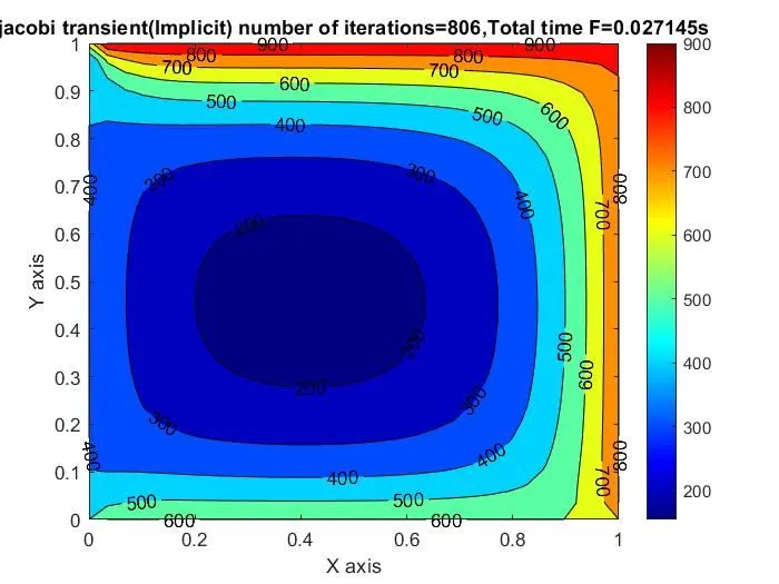
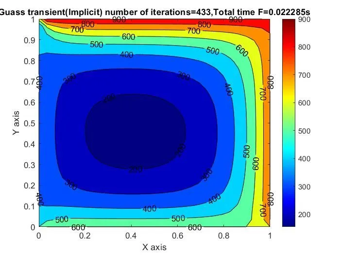
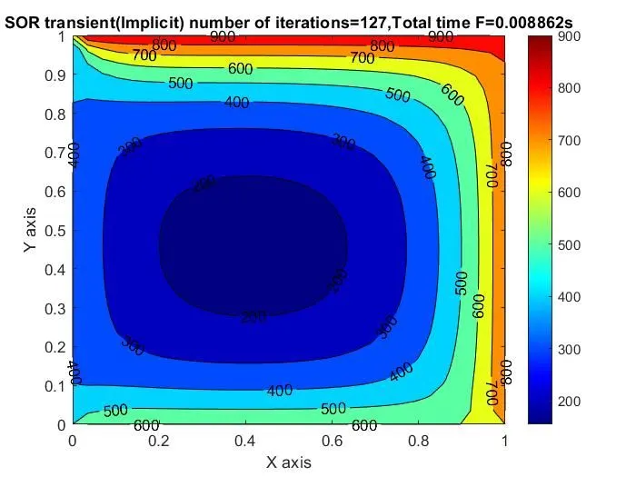
Transient flow (Implicit) output:
RESULTS:
For steady flow
| Method | No. of iterations | Time(Sec) | Error values |
| Jacobi | 1884 | 0.05462 | 9.9772e-05 |
| Gauss-siedel | 1005 | 0.02916 | 9.919e-05 |
| SOR | 101 | 0.00571 | 8.6417e-05 |
For unsteadty flow
| Method | No. of iterations | Time(Sec) | Error values |
| Jacobi | 806 | 0.030935 | 9.963e-05 |
| Gauss-siede | 433 | 0.016274 | 9.769e-05 |
| SOR | 127 | 0.009148 | 9.644e-05 |
From the above results we can conclude that SOR iterative method proves to be solving the converging equation towards the solution at the small time as well as fewer number of iterative cycles with minimum error values.