Week 4 - CHT Analysis on Exhaust port

Aim: To perform steady-state Conjugate Heat Transfer (CHT) analysis on Exhaust port

1. Give a brief description of why and where a CHT analysis is used.
2. Maintain the y+ value according to the turbulence model and justify the results.
3. Calculate the wall/surface heat transfer coefficient on the internal solid surface & show the velocity & temperature contours in appropriate areas.
4. How would you verify if the HTC predictions from the simulations are right? On what factors does the accuracy of the prediction depend on?

Introduction:

Conjugate heat transfer allows simulation of heat transfer between solid and fluid domain by exchanging thermal energies at the interface between them. Some typical turbulence model is used in modelling CHT are laminar, RANS, LES. In solids conduction often dominates and in fluids, convection usually dominates. Efficiently combining heat transfer in solid and fluid is the key to design effective coolers, heaters and heat exchangers. Heat transfer in solid and fluid are combined in a most of application. Typical application of CHT can be performed to improve cooling performance of water jacket and increase engine life. Advancements in cooling for application in gas turbine to understand the complex heat transfer interactions. Critical cooling application involves internal and external film cooling. CHT analysis provides thermal distribution in solid and coolant of engine to provide better insight in velocity distribution and designing thermal load capacity.

Heat Transfer in a Solid:

In most cases, heat transfer in solids, if only due to conduction, is described by Fourier’s law defining the conductive heat flux, q, proportional to the temperature gradient. For a time-dependent problem, the temperature field in an immobile solid verifies the following form of the heat equation.

Heat Transfer in a Fluid:

Due to the fluid motion, three contributions to the heat equation are included:

1. The transport of fluid implies energy transport too, which appears in the heat equation as the convective contribution. Depending on the thermal properties on the fluid and on the flow regime, either the convective or the conductive heat transfer can dominate.
2. The viscous effects of the fluid flow produce fluid heating. This term is often neglected, nevertheless, its contribution is noticeable for fast flow in viscous fluids.
3. As soon as a fluid density is temperature-dependent, a pressure work term contributes to the heat equation. This accounts for the well-known effect that, for example, compressing air produces heat.

Heat transfer co-efficient:

The heat transfer coefficient or film coefficient, or film effectiveness, in thermodynamics and in mechanics is the proportionality constant between the heat flux and the thermodynamic driving force for the flow of heat (i.e., the temperature difference, ΔT):

The overall heat transfer rate for combined modes is usually expressed in terms of an overall conductance or heat transfer coefficient, U. In that case, the heat transfer rate is:

where:

: the surface area where the heat transfer takes place, m²

: temperature of the surrounding fluid, K

: temperature of the solid surface, K.

The general definition of the heat transfer coefficient is:

where:

q: heat flux, W/m²; i.e., thermal power per unit area, q = dQ'/dA

h: heat transfer coefficient, W/(m^2.K)

ΔT: difference in temperature between the solid surface and surrounding fluid area, K

It is used in calculating the heat transfer, typically by convection or phase transition between a fluid and a solid. The heat transfer coefficient has SI units in watts per squared meter kelvin: W/(m²K).

Conjugate heat transfer (CHT):

The Conjugate Heat Transfer (CHT) analysis type allows for the simulation of heat transfer between solid and fluid domains by exchanging thermal energy at the interfaces between them. Typical applications of this analysis type exist as, but are not limited to, the simulation of heat exchangers, cooling of electronic equipment, and general-purpose cooling and heating systems.

The contemporary conjugate convective heat transfer model was developed after computers came into wide use to substitute the empirical relation of proportionality of heat flux to temperature difference with heat transfer coefficient which was the only tool in theoretical heat convection since the times of Newton. This model, based on a strictly mathematically stated problem, describes the heat transfer between a body and a fluid flowing over or inside it because of the interaction of two objects. The physical processes and solutions of the governing equations are considered separately for each object in two subdomains. Matching conditions for these solutions at the interface provide the distributions of temperature and heat flux along the body–flow interface, eliminating the need for a heat transfer coefficient.

Why CHT analysis is used:

Computational Fluid Dynamics (CFD) and more specifically conjugate heat transfer (CHT) analysis can accurately predict heat transfer by simultaneously solving all the relevant solid and flow field heat transfer processes, for example, conduction through solids, free and forced convection in the gases/fluids and thermal radiation.

The CHT approach has an advantage over FE thermal analyses in that wall heat transfer coefficients and their local variations on surfaces are directly calculated within the model rather than based on simplified empirical calculations. The CHT approach, therefore, has benefits for those applications where heat transfer is either non-uniform or difficult to calculate empirically.

Where is CHT analysis used:

Starting from simple examples in the 1960s, the conjugate heat transfer methods have become a more powerful tool for modeling and investigating natural phenomena and engineering systems in different areas of ranging from aerospace and nuclear reactors to thermal goods treatment and food processing, from complex procedures in medicine to atmosphere/ocean thermal interaction in meteorology, and from relatively simple units to multistage, nonlinear processes. A detailed review of more than 100 examples of conjugate modeling selected from a list of 200 early and modern publications shows that conjugate methods are now used extensively in a wide range of applications. That also is confirmed by numerous results published after this book appearance (2009) that one may see, for example, at the Web of Science. The applications in specific areas of conjugate heat transfer at periodic boundary conditions and in exchanger ducts are considered in two recent books.

Solving and modeling approach

• The exhaust port was modeled into the Spaceclaim.
• The exhaust port is a three-dimensional model containing four inlets and one outlet. Despite having isothermal boundary conditions and a uniform flow rate at the four inlets, the model cannot be cut into two halves to save computational time because of its asymmetrical nature. Therefore, the whole model is discretized and is considered for meshing.
• CHT analysis requires both the solid and the liquid volume under consideration, Spaceclaim gives an option of volume extract for selecting edges for fluid volume.
• Both the solid volume and liquid volume are copied into one component.
• Share topology is created.
• Spaceclaim gives an option for share coincident topology, when share coincident topology is selected and executed, the mesh from the fluid volume and the solid volume are said to be conformal with each other which is a requirement for CHT analysis.
• The exhaust port is loaded into the meshing window and then simulated for baseline mesh and the refined mesh.
• The named selections are created ( inlet, outlet, outer wall convection)
• The necessary contour images and graphs are studied to understand the behavior of temperature, velocity, and surface heat transfer coefficient at the interface.

Geometry:

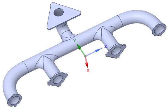
• Load the CAD model of Exhaust manifold in Spaceclaim and check for any extra edges, remove them if any.
• Go to Repair > Volume extract, and select the edges to separate inner and outer volume. Name the outer volume as Solid volume and inner as Fluid volume and move both the volume to new component and delete empty components.
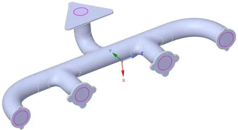
• Go to workbench > Shareprep, to share the physics between the fluid and solid volume and conformal mesh can be achieved and pink circle are seen after completing the process.

Mesh:

Open the mesh tab and select the geometry and named the parts.

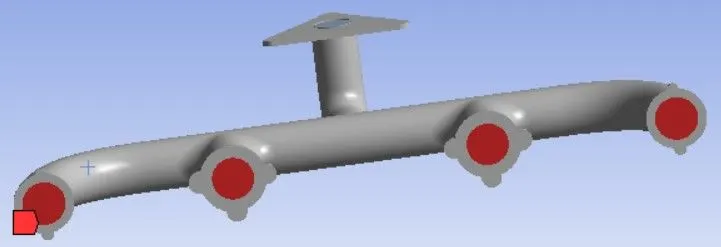
Inlet

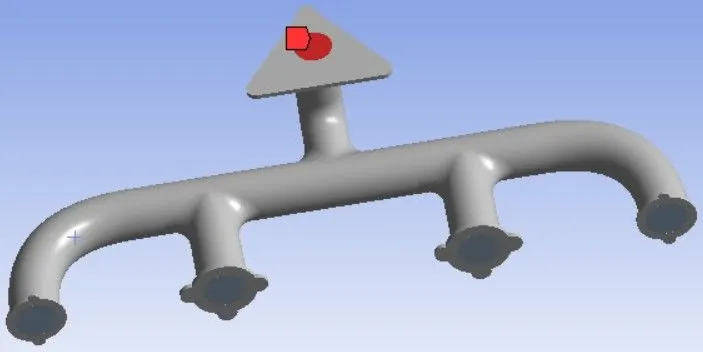
Outlet

Outer-wall-convection

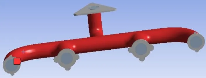
Ansys fluent automaticaly add unnamed part as wall and adiabatic boundary condition is applied.

MESH:

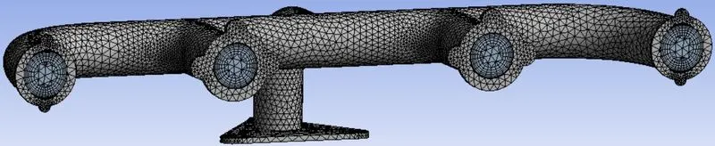
• We are creating the baseline mesh and then we are going to refine the mesh.
• Then go to Mesh>insert>Sizing>Select solid body>assign the element size, and then in the sizing>Advance>curvature capture>yes.
• Then, Mesh>Inflation>Use Automatic inflation>All faces in chosen, and named selection>Select inflation layer, Inflation option>Total thickness, assign the number of layers, growth rate, and the maximum thickness.
• Now, generate the mesh and observing the elements and nodes in the statistics.

Case 1

Element Order: Linear

Element size: 150 mm

Infaltion layer: 5mm

Number of Nodes: 130297

Number of Elements: 388619

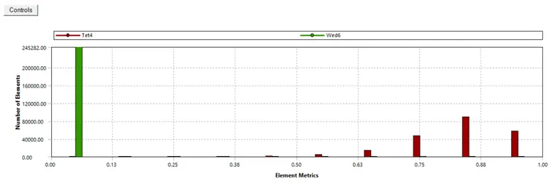
Element Quality

SIMULATION SETUP

1.Solver: Steady

2.Type: Pressure Based

3.Turbulence Model: k-epsilon(Standard)

4.Materials:

• Solid- Aluminium
• Fluid- Air

5.Boundaries:

• Inlet:

Type: Velocity Inlet

Velocity:5 m/s

Temperature:700 K

• Outlet:

Type: Pressure Outlet

Pressure: 0 Pa(Gauge Pressure)

Temperature: 300 K

• Outer-Wall-Convection

Type: Wall

Thermal Conditions: Convection

Heat Transfer Coefficient: 20 W/m2K

Free Stream Temperature: 300K

6. Solution

• Method: Hybrid
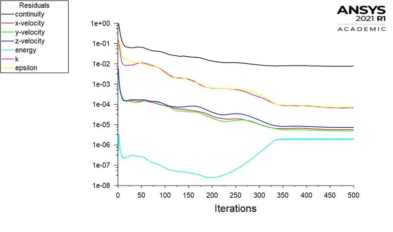
• Number of Iterations: 500

Residuals

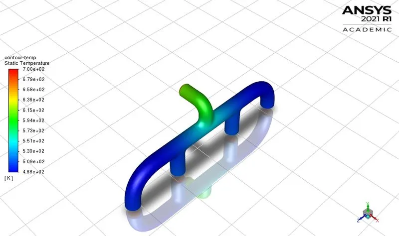
Temperature Contour

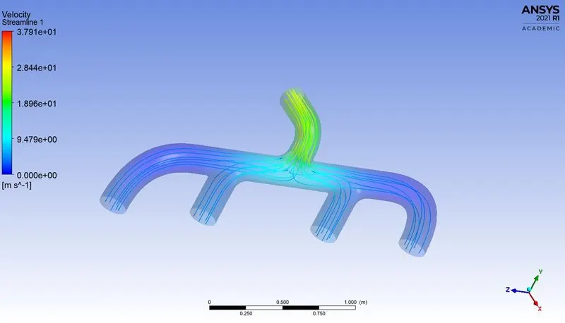
Velocity Streamlines

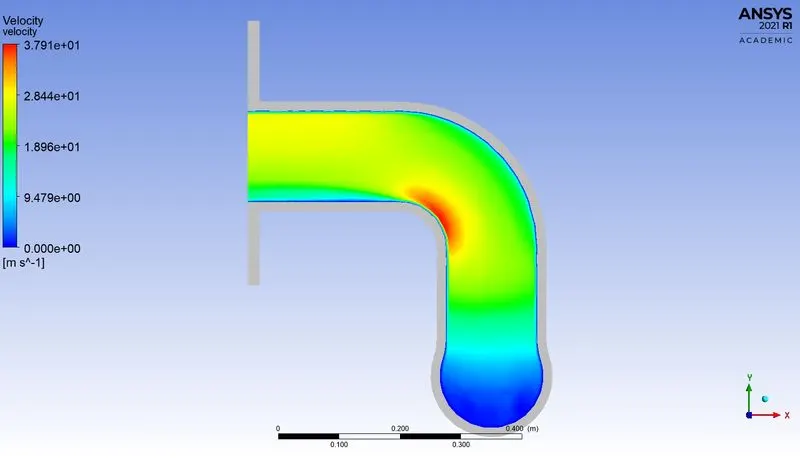
Velocity Contour Along The Outlet

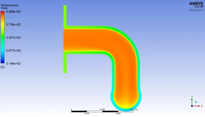
Temperature Contour Along The Outlet

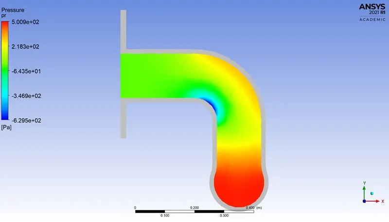
Pressure Contour Along The Outlet

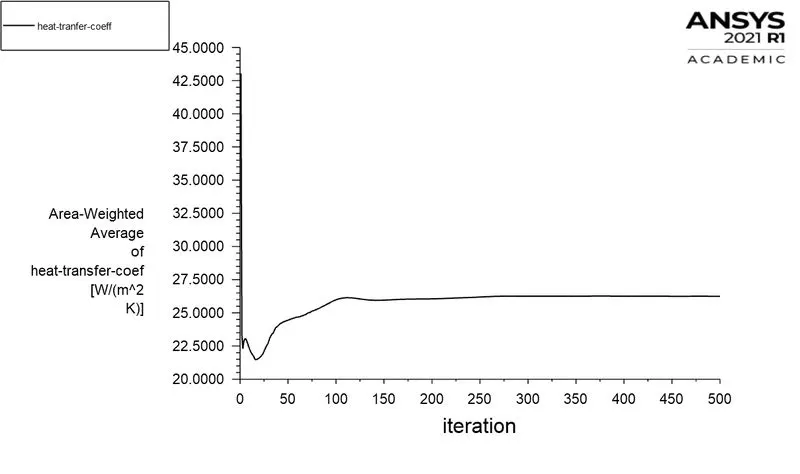
Surface heat transfer co-efficient at outer wall convection

Case 2

Element Order: Linear

Element size: 80 mm

Body size: 10mm

Infaltion layer: 2.5mm

Number of Nodes: 165277

Number of Elements: 456138

Element Quality

SIMULATION SETUP

1.Solver: Steady

2.Type: Pressure Based

3.Turbulence Model: k-epsilon(Standard)

4.Materials:

• Solid- Aluminium
• Fluid- Air

5.Boundaries:

• Inlet:

Type: Velocity Inlet

Velocity:5 m/s

Temperature:700 K

• Outlet:

Type: Pressure Outlet

Pressure: 0 Pa(Gauge Pressure)

Temperature: 300 K

• Outer-Wall-Convection

Type: Wall

Thermal Conditions: Convection

Heat Transfer Coefficient: 20 W/m2K

Free Stream Temperature: 300 k

6. Solution

• Method: Hybrid
• Number of Iterations: 600

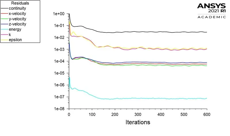
Residuals

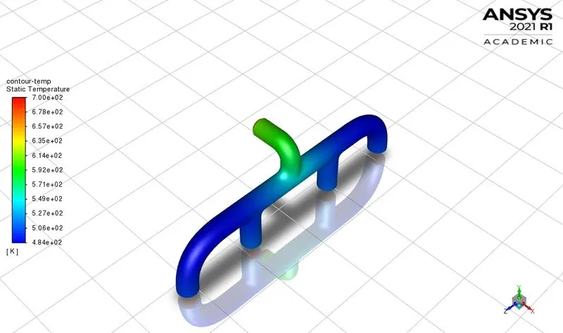
Temperature Contour

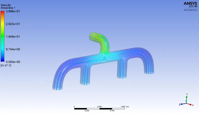
Velocity Streamlines

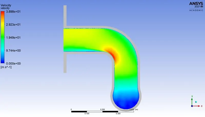
Velocity Contour Along The Outlet

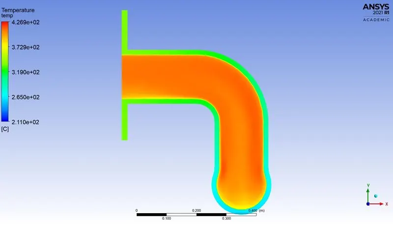
Temperature Contour Along The Outlet

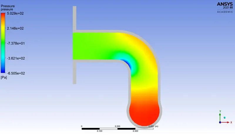
Presssure Contour Along The Outlet

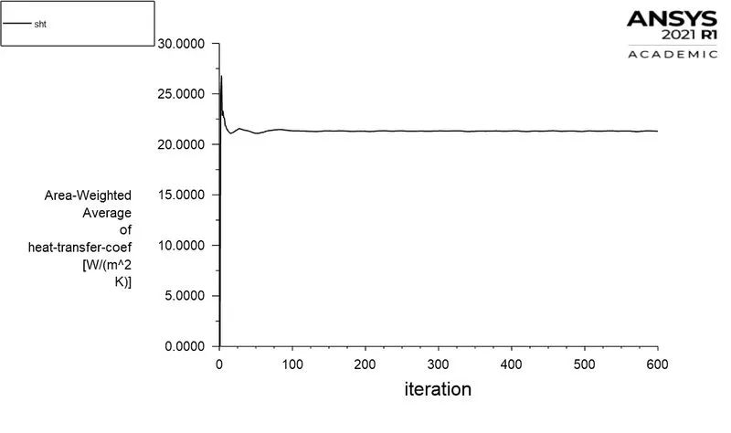
Surface heat transfer co-efficient at inflation layer

How would you verify if the HTC predictions from the simulations are right? On what factors does the accuracy of the prediction depend on?

The typical flow conditions in automotive exhaust systems produce Re numbers in the range of 10^3 to 5*10^4 . The exhaust flow often enters the region Re< 2300, especially in the exhaust manifold runners. In spite of that, the flow remains actually turbulent, since it has flowed through a substantial restriction. The exhaust valves and the persisting, unsteady, flow pulsation effects do not favour the transition to the laminar region

According to the Sieder Tate relation which correlates the Nu number with Re and Pr

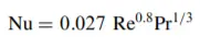
It means Nusselt no. is the function of Reynolds no. and Prandtl no.

As the turbulent boundary layer in the vicinity of bend at outlet port is thin maximum velocity of flow is observed at bend and hence higher Reynold no.

Now, Nu = h*L/K

As Length of pipe and thermal conductivity are constant, value of h will increases as Nu increases and Nu increases as Re increases.

As per our results, heat transfer coefficient is high for higher value of velocity and hence from above discussion we think that our results are correct.

Factors affects the quality of prediction:

• More refined mesh leads to the better results.
• Use inflation layers and apply proper Boundary condition.
• Proper selection of turbulence model according to y+ values.

CONCLUSIONS:

• The velocity tends to increase from the inlet to the outlet because of mass conservation and mixing of air. hence, the high heat transfer coefficient at the junction is due to that high velocity and also when transfer of heat from fluid to solid is high.
• The internal flow velocity and its characteristics are affected by the Initial velocity, Pressure, the physical features of the geometry etc. that affect the heat transfer rates and hence CHT analysis is essential prior experimental analysis for better prediction life of the designed component.
• As shown in the plots, the hot exhaust gases passing through the manifold transfer some of the heat to it via convection. The amount of heat transfer can be related directly with the velocity of the exhaust. The temperature is lower where the flow is stagnate or is moving at the inlet velocity. As the velocity increases, so does the Reynolds number and hence the amount of heat transferred.
• Best methods to predict the accuacy of the result is by comparing the nusselt numbers from experiments and numerical results. The other method to verify is by comparing the results from published experimental results.