Week 8 - Natural Convection-II
Aim: To buid the model for a low-voltage control-panel, as per the given specifications, and perform steady-state thermal analysis of the same.
Introduction:
Low voltage control panel:
A low voltage panel is a component of an electrical distribution system that divides an electrical power feed into branch circuits while providing a protective fuse or circuit breaker for each circuit in a common enclosure. In essence, panelboards are used to protect against electrical overloads and short circuits while distributing electricity throughout a building or facility.
Circuit Breaker:
A circuit breaker is an automatically operated electrical switch designed to protect an electric circuit from damage caused by excess current from an overload or short circuit. Its basic function is to interrupt current flow after a fault is detected. Unlike a fuse, which operates once and then must be replaced, a circuit breaker can be reset (either manually or automatically) to resume normal operation.
Bus bars:
Busbars distribute electricity with greater ease and flexibility than some other more permanent forms of installation and distribution. Sometimes spelled bus bar or bus bar, they are often metallic strips of copper, brass, or aluminum that both ground and conduct electricity.
Objectives:
- The model for a low-voltage control panel is created in ANSYS Icepak using the given specifications
- The computational domain is meshed using non-conformal meshing.
- The model is solved for natural convection.
Geometry:
The complete model of the control-panel is created in ANSYS Icepak using the following steps:
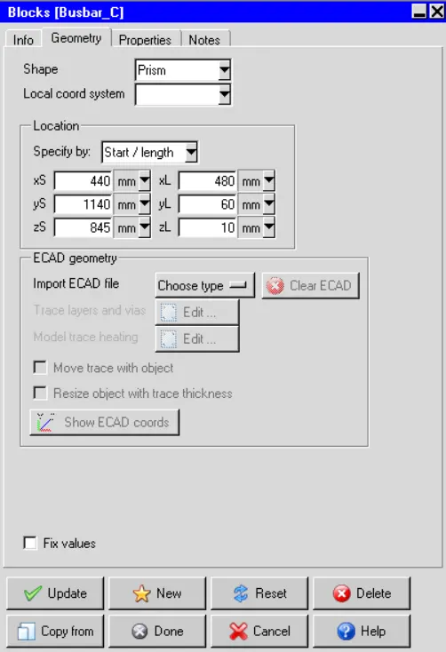
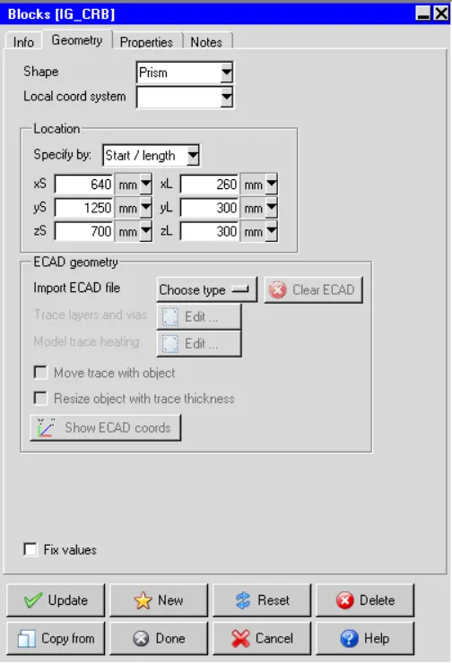
Busbars and circuit-breakers: They form the internal components of the control-panel and are created, as per the given dimensions, using multiple "Blocks" objects available in Icepak. The dimensions and locations of the circuit-breakers are assumed appropriately. The images attached below show the geometry settings used to define one of each of the busbars and the circuit-breakers.
- Busbar_C
ii. Circuit-breaker IG
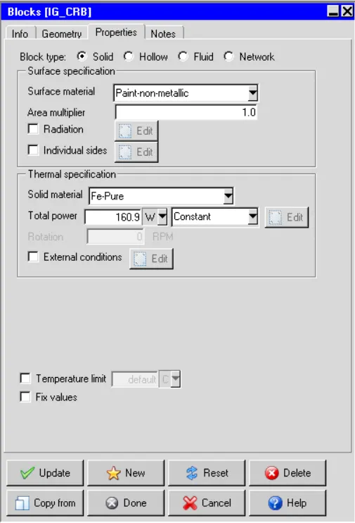
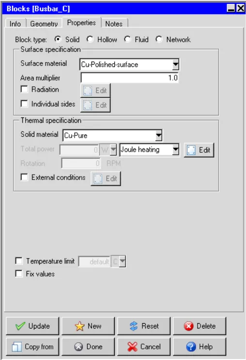
All the internal components (busbars and cables are assigned the same solid material ("Cu-Pure") and surface material ("Cu-polished-surface") except circuit breakers
The images attached below show the settings applied in the "Properties" tab to define one of each of the busbars and the circuit-breakers
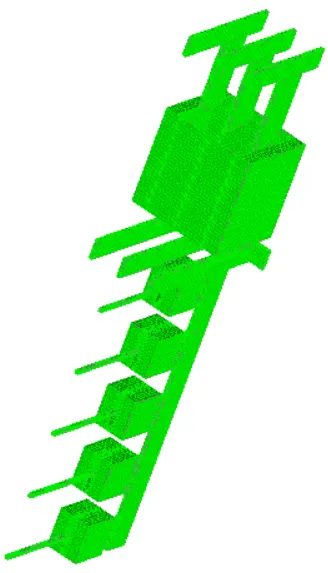
The image attached below shows all the busbars and circuit-breakers that are located within the control-panel.
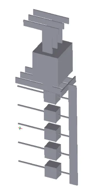
Control-panel: It houses the current carrying components (busbars) and circuit-breakers and is created using the "Enclosure" object available in Icepak, as per the given outer dimensions. "Steel-Carbon-1020" and "Paint-white-acrylic" are used as the solid material and the surface material respectively, for the control-panel. Each wall of the control-panel is assigned a "Thin" type boundary condition and a thickness of 2 mm. Radiation heat transfer is enabled for all the walls of the control-panel. The images attached below show the settings applied in the "Geometry" and "Properties" tabs, to define the control-panel.
i. Geometry
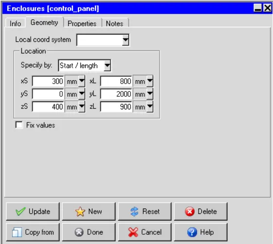
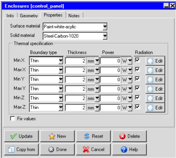
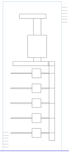
Two grilles are defined on a pair of opposite walls of the control-panel to allow: the ambient air to move into the control-panel and the air inside the control-panel to move out of it. The grille for the intake of ambient air is placed near the base of the control-panel while the grille for the output of hot air is placed near the top of the control-panel. Hence the two grilles allow air-cooling of the heat generating components (located inside the control-panel) due to natural convection. The image attached below shows the control-panel.
Meshing
The following meshing techniques are utilized in the current project to discretize the computational domain:
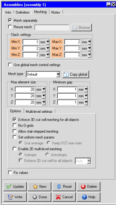
1. Non-conformal meshing technique allows the user to selectively refine the mesh within a sub-region around an assembly by selecting the "Mesh separately" option available in the "Meshing" tab of the assembly settings. A comparatively coarse mesh can be used for the rest of the model. Multiple assemblies, that employ non-conformal meshing, are defined in the model. The image attached below shows the settings applied in the "Meshing" tab to define one such assembly.
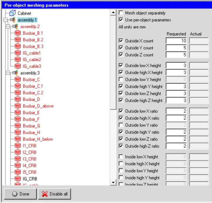
2. The "Object params" option available in the "Mesh control" window allows the user to refine the mesh locally near one or more objects/assemblies defined in the model. "Per-object meshing parameters" are specified for the assembly defined around the control-panel in the current model. The image attached below shows the settings applied in the "Per-object meshing parameters" window for the assembly.
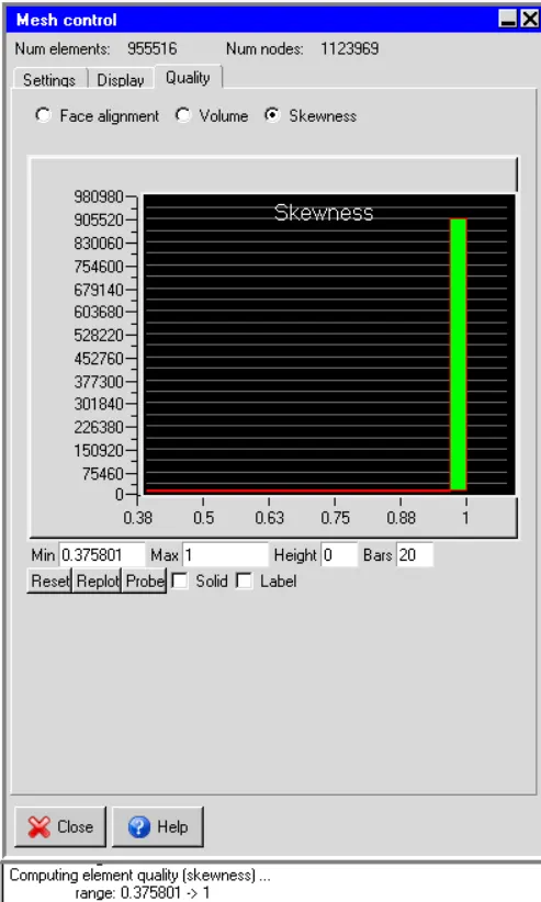
After completing the above steps, the computational mesh is generated. The image attached below shows the "Mesh control" window.
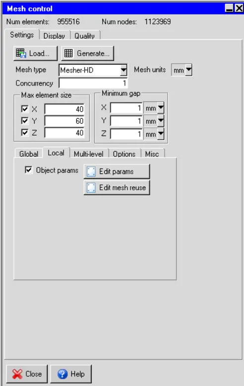
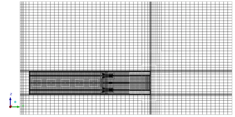
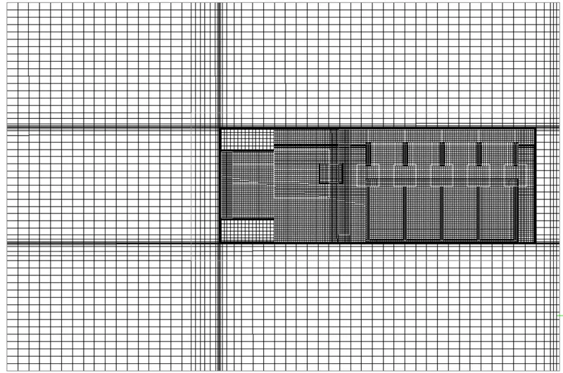
The image shows that the generated mesh yields 955516elements and 1123969 nodes. The images attached below show the computational mesh on three mutually perpendicular planes, each passing through the center of the cabinet.
i. X-plane
ii. Y-plane
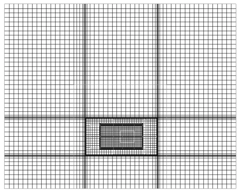
iii. Z-plane
The images attached below show the volume mesh on the components located inside the control-panel: busbars and circuit-breakers.
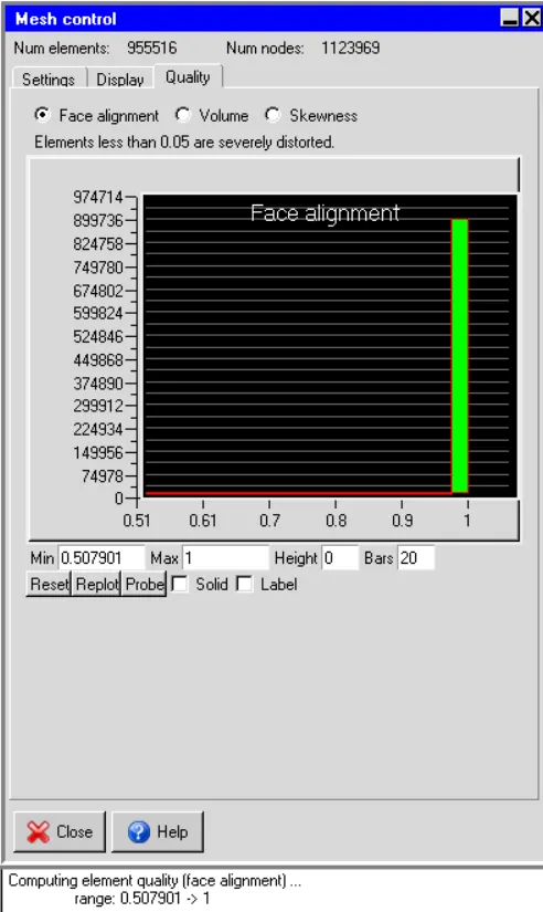
Visually the mesh appears to be fine. The images attached below show the histograms with the number of elements plotted along the X-axis and the quality measures plotted along the Y-axis.
1. Face alignment 2. Skewness
Solver:
The three-dimensional steady-state Navier-Stokes equations for the model are solved within the computational domain using the Fluent solver available in ANSYS Icepak. The following settings are applied to the solver:
1. Variables solved: Flow (velocity, pressure) and Temperature
2. Radiation: On
2.1. Model: Surface to surface radiation model
3. Flow regime: Turbulent
3.1. Model: Zero equation model
4. Time variation: Steady
5. Solution initialization
5.1. X velocity: 0
5.2. Y velocity: 0.000980665 m/s
5.3. Z velocity: 0
5.4. Temperature: Ambient (20 deg. C)
6. Natural convection
6.1. Density model: Boussinesq approximation
6.2. Operating pressure: 101325 N/m2
6.3. Operating density: 1.225 Kg/m3
6.4. Gravity vector: 9.80665 m/s^2 directed along the negative Y-axis
7. Number of iterations: 1000
8. Convergence criteria
8.1. Flow: 1e-7
8.2. Energy: 1e-7
8.3. Joule heating: 1e-7
9. Configuration: Parallel
10. Number of processors: 4
11. GPU computing: Enabled
12. Number of GPUs: 1
13. Discretization scheme
13.1. Pressure: Standard
13.2. Momentum: First
13.3. Temperature: First
14. Under-relaxation factors
14.1. Pressure: 0.3
14.2. Momentum: 0.7
14.3. Temperature: 1
14.4. Viscosity: 1
14.5. Body forces: 1
14.6. Joule heating potential: 1
15. Linear solver settings
15.1. Pressure - Type: V, Termination criterion: 0.1, Residual reduction tolerance: 0.7, Stabilization: None
15.2. Momentum - Type: flex, Termination criterion: 0.1, Residual reduction tolerance: 0.7
15.3. Temperature - Type: F, Termination criterion: 0.1, Residual reduction tolerance: 0.7, Stabilization: None
15.4. Joule heating potential - Type: F, Termination criterion: 0.1, Residual reduction tolerance: 0.7, Stabilization: None
16. Precision: Double
Results:
In the current section, the simulation results are discussed.
1. Residuals:
The residuals of the following equations are plotted against the number of iterations:
i. Continuity equation
ii. X-Momentum equation
iii. Y-Momentum equation
iv. Z-Momentum equation
v. Energy equation
The image attached below shows the residuals plotted against the number of iterations.
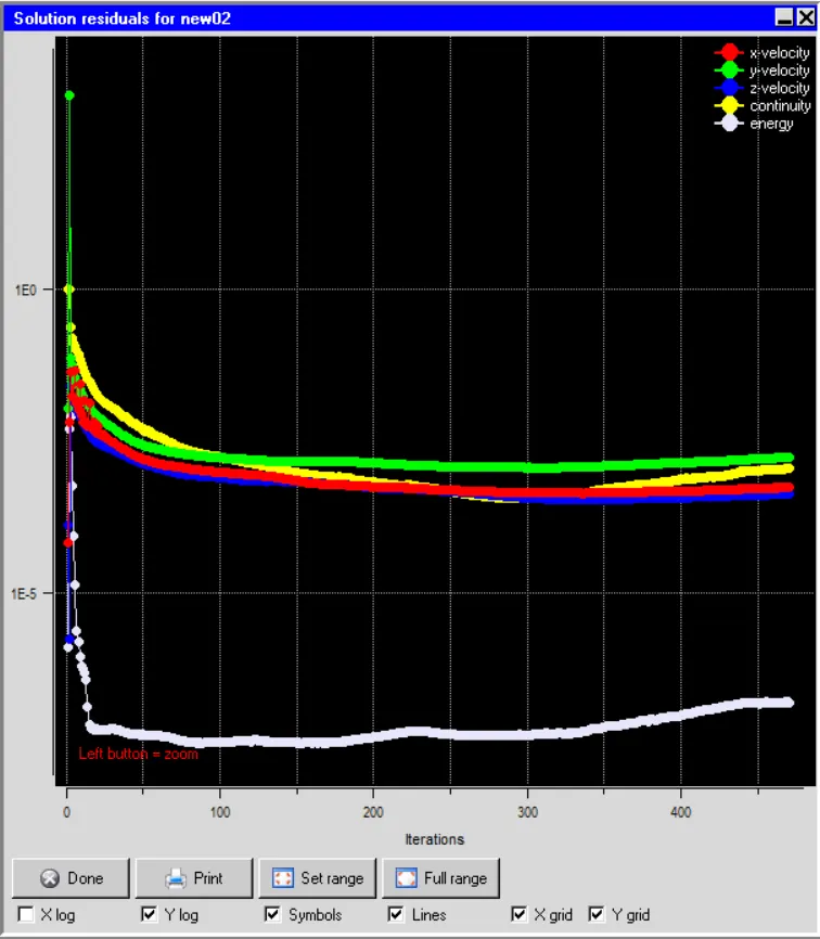
The solution got converged about 450 iterations
Velocity contours:
The steady-state velocity contours are plotted on the X-plane passing through the center of the cabinet, as shown in the image attached below.
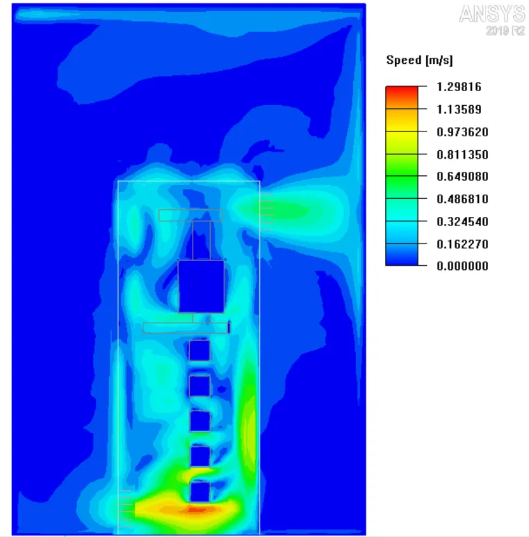
The plot shows that the air within the computational domain is in a state of motion. This can be attributed to natural convection which drives the air upwards, against the gravitational field, due to the difference in density created by the virtue of temperature difference. According to the contour-legend the maximum air-velocity on the X-plane passing through the center of the cabinet is 1.2 m/s.
Velocity vectors:
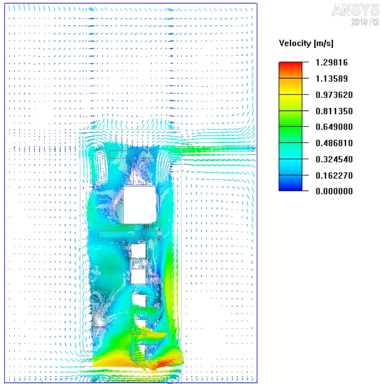
The steady-state velocity vectors are plotted on the X-plane passing through the center of the cabinet, as shown in the image attached below.
Temperature contours:
The steady-state temperature contours are plotted on the X-plane passing through the center of the cabinet, as shown in the image attached below.
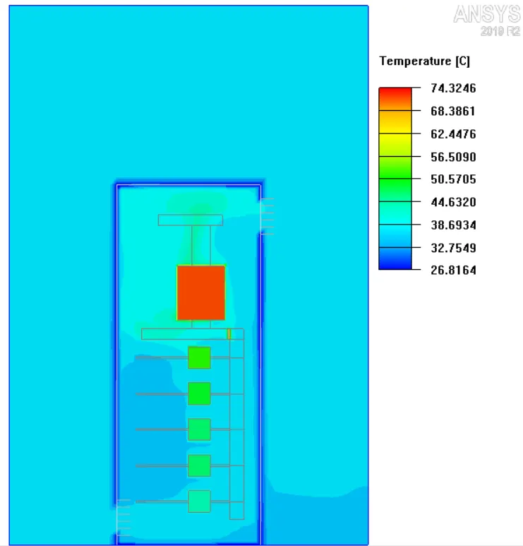
The plot shows that the air within the computational domain is cooler than any other object. It can be seen that the temperature of the air within the computational domain increases as we move up (against gravity). This can be explained in the following manner: the air that is in direct contact with the comparatively hotter objects takes up their heat due to which its temperature increases and its density decreases. Under the influence of the downward gravitational field, this lighter (hotter) air rises up and the surrounding heavier (cooler) air rushes in to fill up the evacuated space.
Object face temperature contours:
The steady-state temperature contours are plotted on all the objects in the model that are located inside the control-panel (the busbars and the circuit-breakers), as shown in the image attached below.
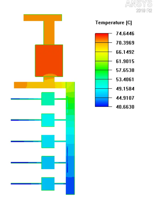
The contours show that the circuit-breaker IG attains the highest steady-state temperature, followed by busbar-B, busbar-C, the remaining circuit-breakers and the remaining busbars respectively.
Particle traces:
The steady-state particle traces (colored by temperature) of 100 particles that originate at the lower grille of the control-panel are plotted within the computational domain, as shown in the animation attached below.
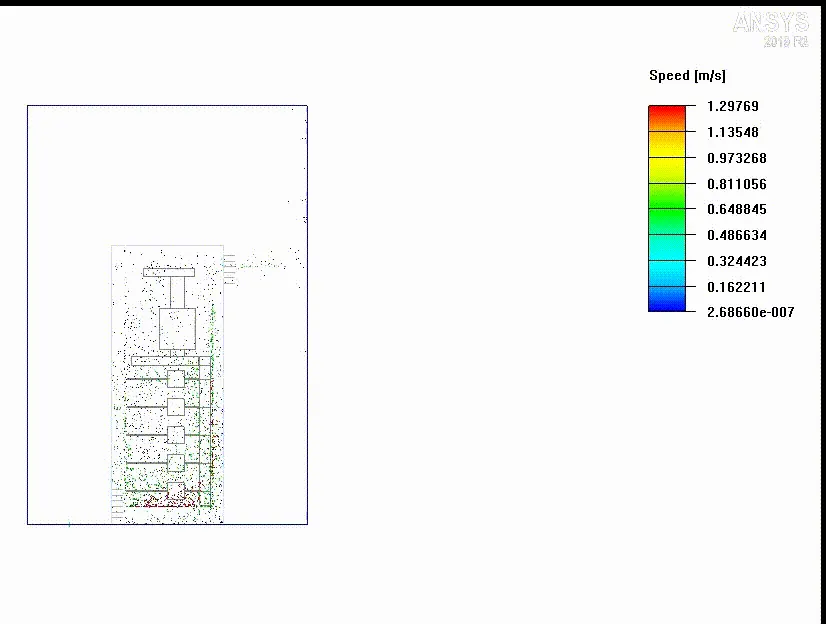
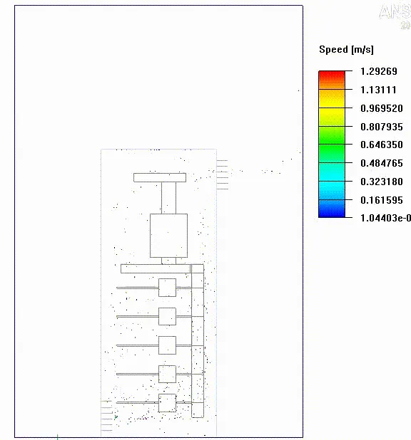
The animation clearly shows the steady-state pathlines traced by air particles, that originate at the lower grille of the control-panel, within the computational domain. The color of a pathline at a particular location indicates the temperature of the air particle that traces the pathline, at that location.
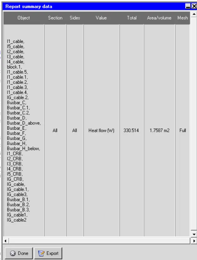
Heat flow:
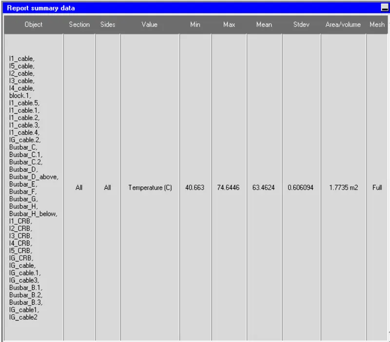
Temperature:
Conclusion:
In the current project, the model of a low-voltage control-panel was created in ANSYS Icepak using the given design-specifications. The model was meshed using the following features available in the Icepak mesher: non-conformal meshing and per-object meshing parameters. The solver was setup using suitable settings to incorporate the following physical phenomena:
i. Joule heating
ii. Natural convection
iii. Turbulence
iv. Radiation heat transfer
The three-dimensional steady-state governing equations for the model were solved for flow and thermal fields within the computational domain using the Fluent solver available in ANSYS Icepak. The following conclusions can be drawn based on the simulation results:
i. According to the steady-state velocity contours, the maximum velocity within the computational domain is 1.2 m/s.
ii. The highest steady-state temperature within the computational domain is attained by the circuit-breaker IG and its numerical value is 74.64 °C.