Week 4.2: Project - Transient simulation of flow over a throttle body
Aim:
To perform a Transient simulation of flow over a throttle body in Converge 3.0
Objective:
- Setup and run transient state simulation for flow over a throttle body.
- Post-process the results and show pressure and velocity contours.
- Show the mesh (i.e surface with edges)
- Show the plots for pressure, velocity, mass flow rate, and total cell count.
- Show the calculations on how you calculated an end time for the simulation.
- Create an animation in which its throttle movement should be visible.
Introduction:
Throttle:
A throttle is a mechanism by which the fluid flow is managed by construction or obstruction. An engines power can be increased or decreased by the restriction of inlet air due to the presence of throttle. The term throttle can be used to increase the efficiency of the car, the car accelerator peddal can be used as throttle to increase the efficiency of the engine. It is used as throttle in the field of aviation, known as thrust lever in jet engine powered aircraft. For steam locomotive the valve which controls the regulation of gas is called as reguator.
Application of throttle:
The throttle is a mechanism which is used to increase or decrease the power of engine by restricting the flow of inlet gases coming through it. There are numerous applications of the throttle mechanism which are listed below
- Internal Combustion Engines
- Fuel Injected Engines
- Reciprocating Engine Aircraft
- Steam locomotives
- Automobiles
CFD Modelling:
The flow chart or the procedure is
- Creating Geometry / Importing Geometry
- Debugging the geometry if any
- Boundary flagging or creating boundaries
- Case set up
- running the simulation and post processing.
Geometry:
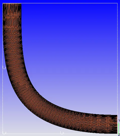
The geometry used for performing simulation is attached below.
Case Setup:
First we need to choose the Application type as Time based.
Material
Air (Predefined mixture) is used as the working fluid for performing gas simulation. Accordingy, the following global properties are utilized:
Global transport equation:
Turbulent Prandtl number: 0.9
Turbulent Schmidt number: 0.78
Species:
Add the O2 and N2 in the species.
Simulation parameters:
Run Parameters:
Solver - Transient
Simulation mode - Full hydrodynamic
Gas Flow Solver - Compressible
Uncheck steady state monitor under misc tab
Simulation time parameters:
Start time - 0 cycles
End time - 0.01 cycles
Initial time step - 1e-9 s
Minimum time step - 1e-9 s
Maximum time step - 1 s
Maximum Convection CFL limit - 1
Solver Parameters:
Solver scheme - PISO
Solver type - Pressure based
Boundary conditions:
The following boundary conditions are applied:
1. Inlet: INFLOW type boundary condition is applied with the following settings:
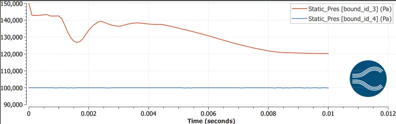
Total pressure: 151987.5Pa
Velocity: Zero normal gradient
Temperature: 300K
Species: Mass fractions: Oxygen: 0.23; Nitrogen: 0.77
Turbulent kinetic energy (tke): Intensity=0.02 (fraction)
Turbulent dissipation (eps): Length scale=0.003m
2. Outlet: OUTFLOW type bundary condition is applied with the following settings:
Pressure: 101325Pa
Velocity: Zero normal gradient
Temperature backflow: 300K
Species backflow: Mass fractions: Oxygen:0.23; Nitrogen: 0.77
Turbulent kinetic energy (tke) backflow: Intensity=0.02 (fraction)
Turbulent dissipation (eps) backflow: Length scale=0.003m
3. Elbow_wall: WALL type boundary condition is applied with the following settings:
Wall motion type: Stationary
Surface movement: FIXED
Velocity: Law of wall
Temperature: Law of wall; 300K
Turbulent kinetic energy (tke): Zero normal gradient
Turbulent dissipation (eps): Wall model
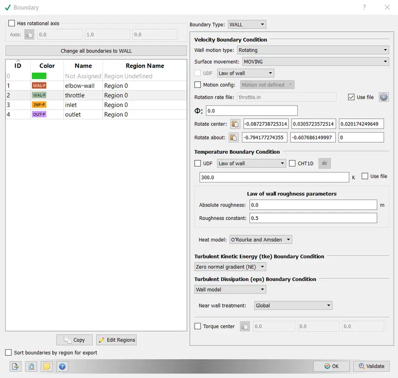
4. Throttle: WALL type boundary condition is applied with the following settings:
Throttle movement profile:
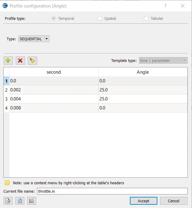
After assinging the boundary conditions we need to assign the regions for all the boundaries.
We need to create a region to initialize the setup.
The initial pressure and then the Inlet pressure should have to be same.
Grid:
Computational grid with the following features is used for performing simulation:
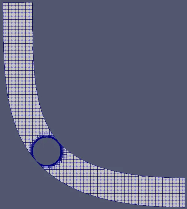
i. Base grid size: dx=dy=dz=0.002m.
ii. Fixed embedding: Enabled; Entity type: Boundary; Boundary ID: Throttle; Mode: PERMANENT, Scale: 3, Embed layers: 2
After that we need to select the RNG turbulence model.
Output/Post processing
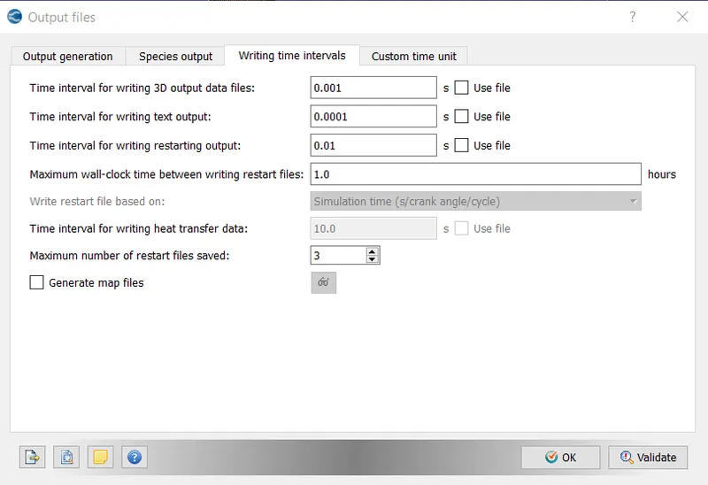
In this part we need to choose the variable which we want to plot.
Solution:
- After setting up the case in Converge, we have to save the setup file
- Aftet that we have to export the input files.
- After exporting the files we have to open CYWIN to perform the simulation.
- In the CYGWIN, we need to choose the directory at where we exported the input files.
- Then we have to copy and paste the location of intelmpiconverge.exe
The figure attached below shows the computational grid
Results
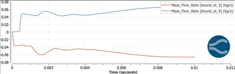
1. Mass flow rate
Mass flow rate at inlet and outlet is plotted over time.
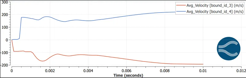
2. Average velocity
Average velocity at inlet and outlet is plotted over time.
3. Static pressure
Static pressure at inlet and outlet is plotted over time.
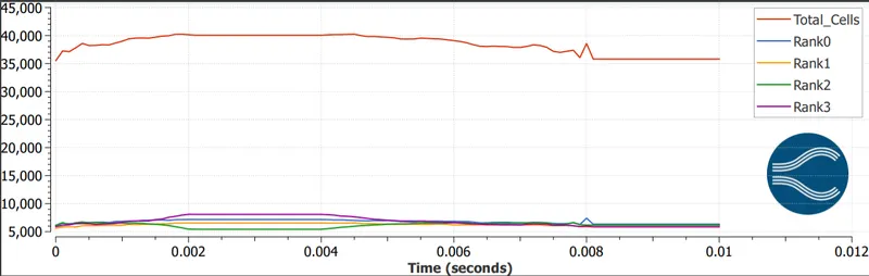
4. Cell count ranks
Cell count ranks are plotted over time. Since the mesh keeps changing with time, due to throttle movement, the cell count is also not constant.
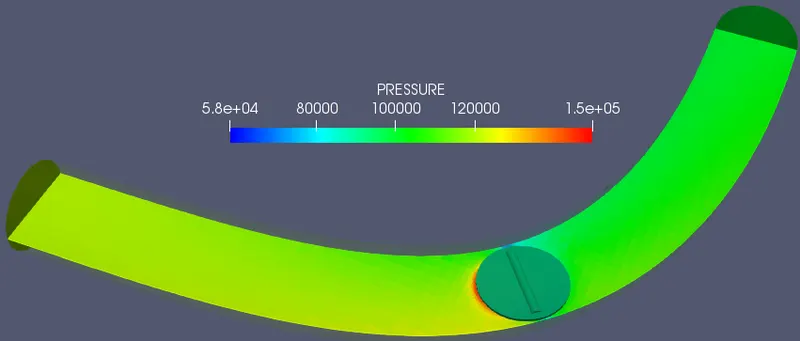
Pressure contours:
Pressure contours are plotted over a cut-plane at t=10ms.
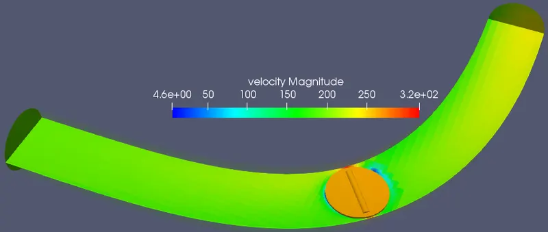
Velocity contours:
Velocity contours are plotted over a cut-plane at t=10ms.
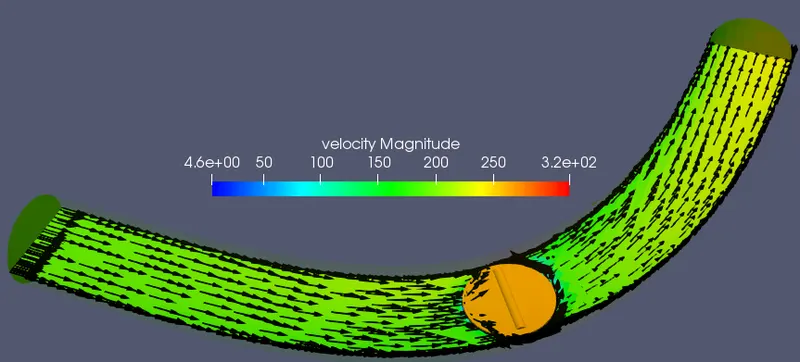
Velocity vectors:
Velocity vectors are plotted over a cut-plane at t=10ms.
Animations:
Velocity contours
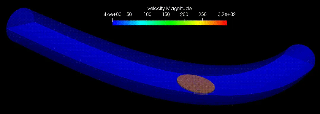
The animation attached below shows the evolutionof velocity contours on a cut-plane with time.
Conclusion:
1. The plot for mass flow rate indicates a good mass balance between inlet and outlet.
2. The plot for average velocity shows that the average velocity at the outlet (at t=10ms) is 226.286m/s.
3. Pressure contours show maximum and minimum pressure values near the upstream and downstream locations of the throttle valve respectively.
4. Velocity contours show that a maximum velocity of 330m/s is achieved in the passage between throttle valve and pipe.
5. The animations show the influence of throttle movement on the nearby velocity field and streamlines