Week 12 - Final Project - Modelling and Analysis of a Datacenter

Aim:The objective of this challenge is to model a replica of the datacentre where high power distribution units are working and to analyze the flow distribution and behavior of the temperature of server stacks inside the datacentre.

Given:

Problem Description:

This tutorial considers a 1200 sq. ft. datacenter with a slab to slab height of 12 ft. The datacenter consists of a 1.5 ft underfloor plenum and a 2 ft ceiling plenum. The CRACs discharge cold air into the underfloor plenum. The cold air enters the main datacenter space mainly through the perforated floor tiles and returns back to the air conditioning units. The cooling load, as summarized as below. Size and Capacity of Heat Sources in Datacenter corresponds to the heat output from the server cabinets and the PDUs. A PCB board, library files and traces are imported to create the model. The model is first solved for conduction only, without the components and then solved using the actual components with forced convection.

Heat Source	Size	Power
Server Cabinet	2 ft x 3 ft x 7 ft	3000 W
High Density	2 ft x 3 ft x 7 ft	7000 W
PDU	4 ft x 2 ft x 5 ft	3600 W

Introduction:

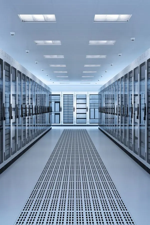
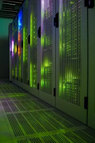
Data centers are simply centralized locations where computing and networking equipment is concentrated for the purpose of collecting, storing, processing, distributing or allowing access to large amounts of data. They have existed in one form or another since the advent of computers.

Because of their high concentrations of servers, often stacked in racks that are placed in rows, data centers are sometimes referred to as a server farm. They provide important services such as data storage, backup and recovery, data management, and networking. These centers can store and serve up Web sites, run e-mail and instant messaging (IM) services, provide cloud storage and applications, enable e-commerce transactions, power online gaming communities and do a host of other things that require the wholesale crunching of zeroes and ones.

The sole purpose of data center cooling technology is to maintain environmental conditions suitable for information technology equipment (ITE) operation. Achieving this goal requires removing the heat produced by the ITE and transferring that heat to some heat sink.

Geometry:

• Used the inbuilt option called macros to model the components in the datacenter.
• Ansys Icepak includes many macros designed to automate common model-building tasks. Macros are available to assist with creating different types of packages, PCBs, heat sinks, heat pipes, thermoelectric coolers, JEDEC test configurations, and DELPHI package characterization.
• Hereby using the macros, we have modeled the computer room air conditioning units (CRACs), server cabinets, power distribution units (PDUs), and perforated floor tiles.

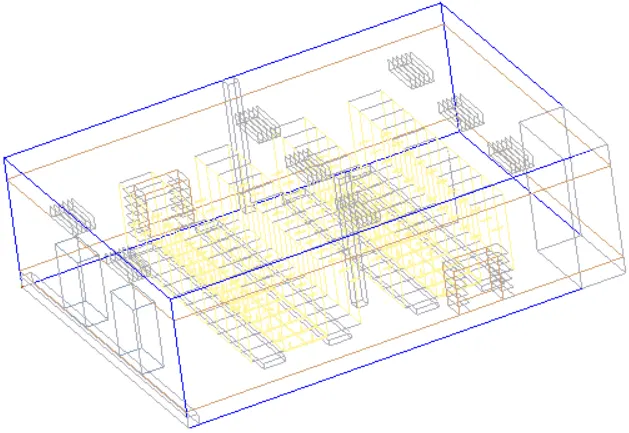
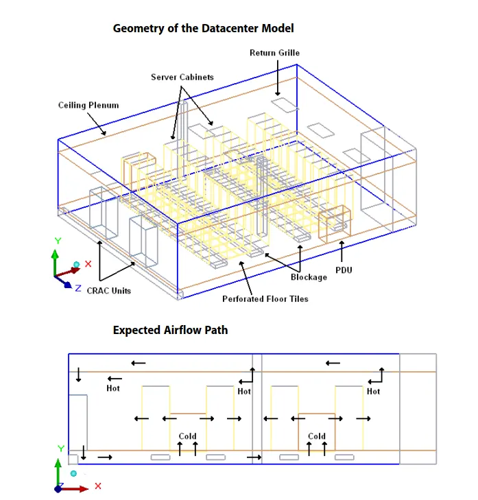
• The above figure shows what are the parts we have modeled and where we positioned them. The picture right below it says the direction of the flow of air (hot & cold).

Meshing:

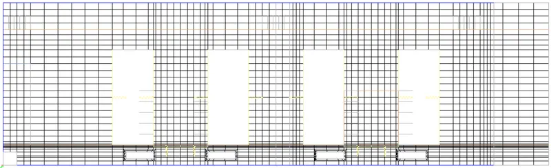
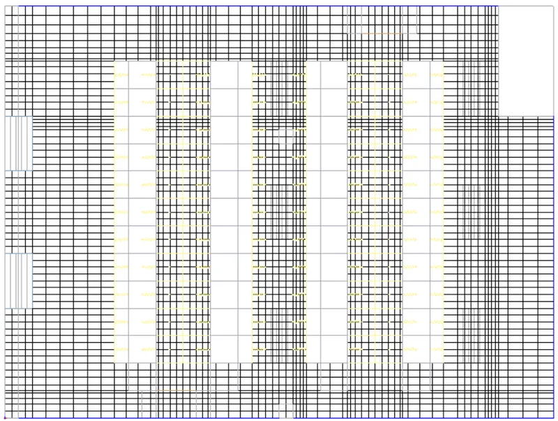
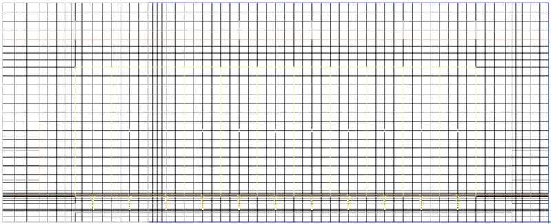
The computational domain is discretized using the Hex-dominant grid generated by the "Mesher-HD". The maximum element sizes along the X, Y and Z directions are set to 2 ft, 0.5 ft and 1 ft respectively. The minimum gaps along the X, Y and Z directions are set to 1 in, 0.36 in and 0.01 in respectively. The image attached below shows the "Mesh control" window.

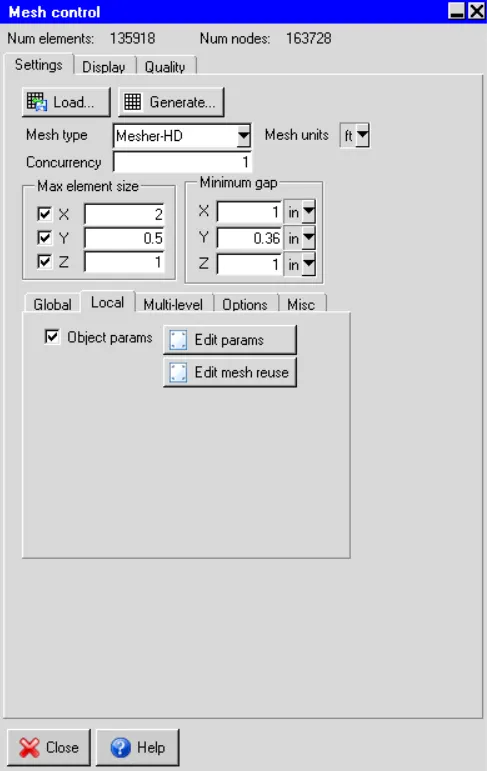
• The maximum element size taken is 1 * 0.5 * 1 inch. The minimum element size taken is 1 * 0.15 * 1 inch.
• A Mesher-HD mesh type is used to generate the mesh.
• The number of elements generated is 135918 and the number of nodes generated is 163728.
• Normal mesh parameters are used to generate the mesh.
• Object parameters are applied to the geometry to generate the mesh.

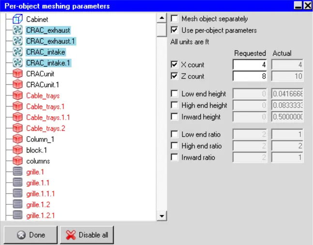
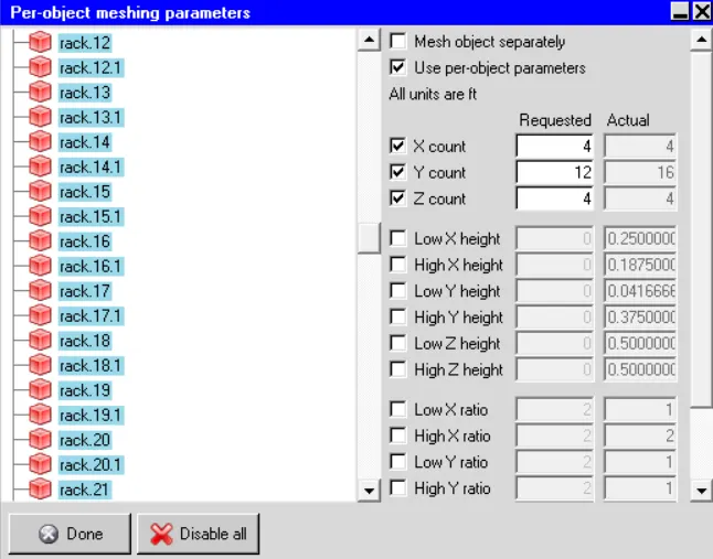
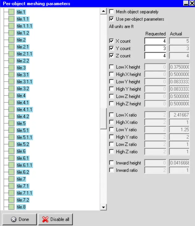
• Here the objects colored with red color are given with per-object parameters. This per-object parameter concept is used to generate a fine mesh without any overlaps of the elements.
• The object parameters will help us to generate more amount of elements and nodes so that we will capture physics accurately at some particular places like PDU's, CRAC's, tiles, etc.

Z-plane:

Y-plane:

X-plane:

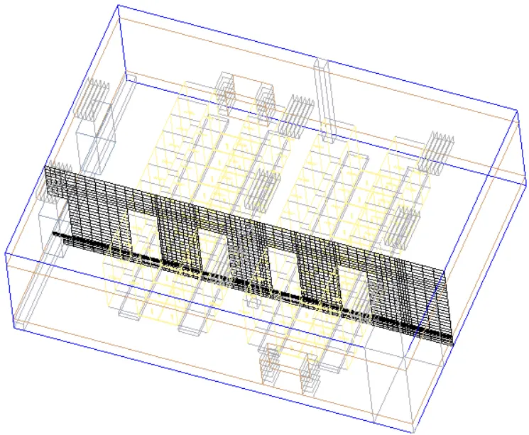
Visually the mesh appears to be fine. The images attached below show the histograms with the number of elements plotted along the X-axis and the quality measures plotted along the Y-axis.

1. Face-alignment

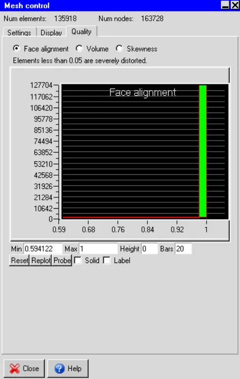
Values less than 0.05 indicate the presence of severely distorted elements in the mesh.

2. Volume

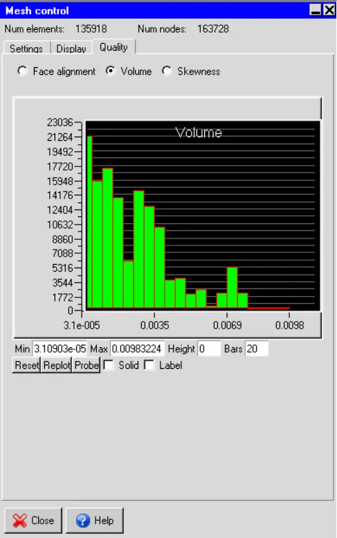
For a double precision solver the minimum cell volume should not be less than 1e-15 m^3 otherwise the solver may face issues.

3. Skewness

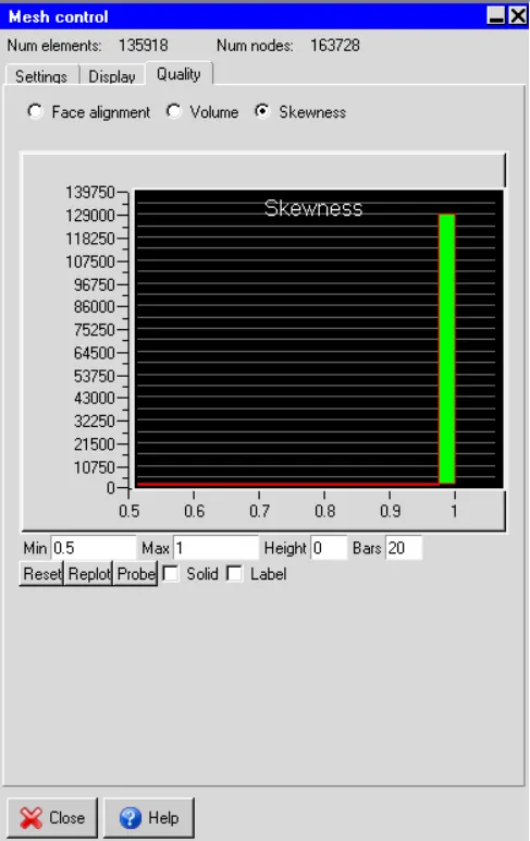
A skewness of 0 indicates that the mesh element is degenerate whereas a skewness of 1 indicates that it is ideal (equilateral/equiangular).

Solver:

The three-dimensional steady-state Navier-Stokes equations for the model are solved within the computational domain for flow and temperature field using the Fluent solver available in ANSYS Icepak

Numerical setting:

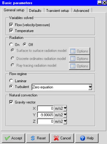
Basic parameters:

• In the basic parameters where we have given whether the solution runs for temperature, flow, and setting up for the initial temperature as well as radiation temperature, etc..
• Here we are solving both the flow and temperature variables for the modeled geometry.
• We are neglecting the radiation effect because we are interested in solving major heat transfer spots.
• The turbulent model we are calculating is Zero-equation.
• A turbulent flow regime has to be calculated with the gravity vector of -9.81 m/s in Y-direction in the natural convection space.
• Internal convection usually cannot be treated using simple boundary layer theory because the entire fluid in the enclosure engages to the convection.
• When heat is added to a fluid and the fluid density varies with temperature, a flow can be induced due to the force of gravity acting on the density variations. Such buoyancy-driven flows are termed natural-convection (or mixed-convection) flows and can be modeled by ANSYS FLUENT.

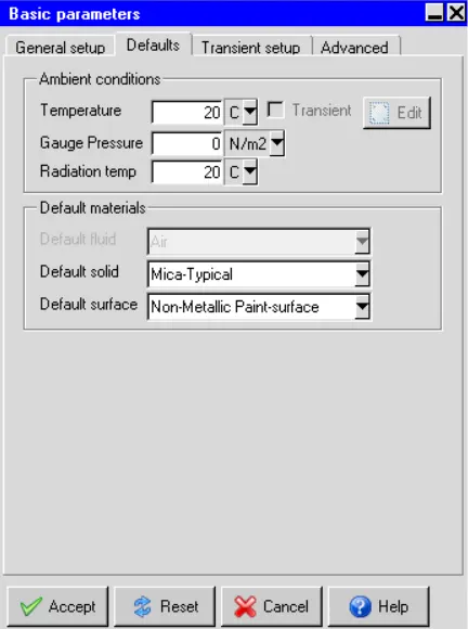
• The temperature conditions maintained inside are ambient in nature, which is 20 degrees centigrade.
• The solid materials used in the model are Mica-Typical.In the electrical industry the same as thermal insulation, and electrical insulators in electronic equipment.
• The surface material used is Paint-non metallic.
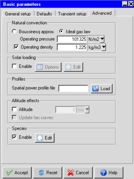
• Here we have enabled the species section and provided the H2O gas as a species inside the model of the datacenter.

Basic Settings:

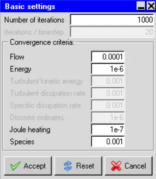
• Here in the basic settings panel, we need to give the number of iterations to 1000.
• The convergence criteria of Flow is set to 0.0001 and energy is set to 1e-6, turbulent kinetic energy to 0.001, and joule heating is set to 1e-7.

Advanced settings:

• Here in this panel, we give the inputs as the discretization schemes for the pressure, momentum, and temperature are of the first order.
• The double precision is given. Single precision means that the floating-point numbers will be represented in a 32-bit system whereas double-precision means that they will be represented in a 64-bit system. So Calculation in double precision will be more accurate.

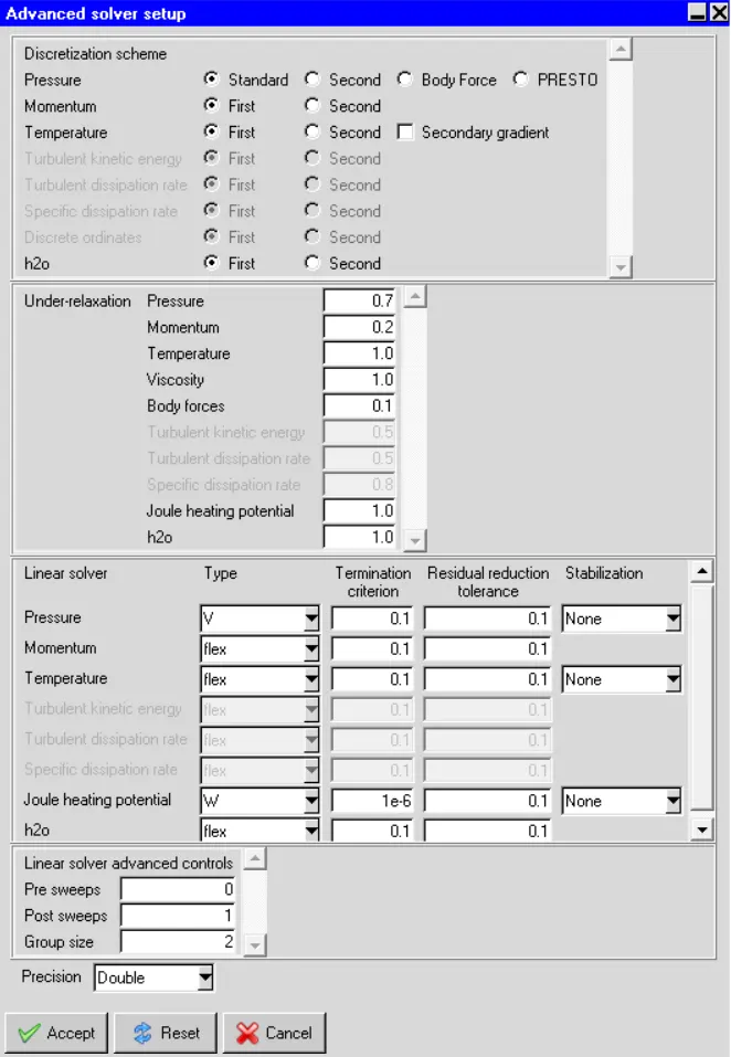
• We have adjusted the under relaxation factors of momentum and body force for the convergence criteria.

Results:

In the current section, the simulation results are discussed.

Residuals:

The residuals for the energy equation are plotted against the number of iterations, as shown in the image attached below.

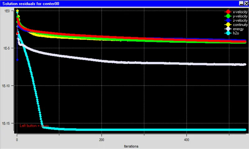
• From the above residual plot, we have seen that the solution gets converged, and we didn't find any kind of instability of the iterations of pressure, momentum, and energy in the residual plot.
• At the same time the velocity, continuity, and energy equation are well below the ranges we applied in the basic setting of iterations. Which means the solution gets very well converged.

Monitor Points:

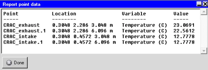
Temperature monitor points are created within the computational domain not only to monitor the steady-state temperatures of the key objects in the model, such as heat sources and heat sinks, but also to inform the advent of steady state. The image attached below shows the data recorded by the temperature monitor points plotted against the number of iterations.

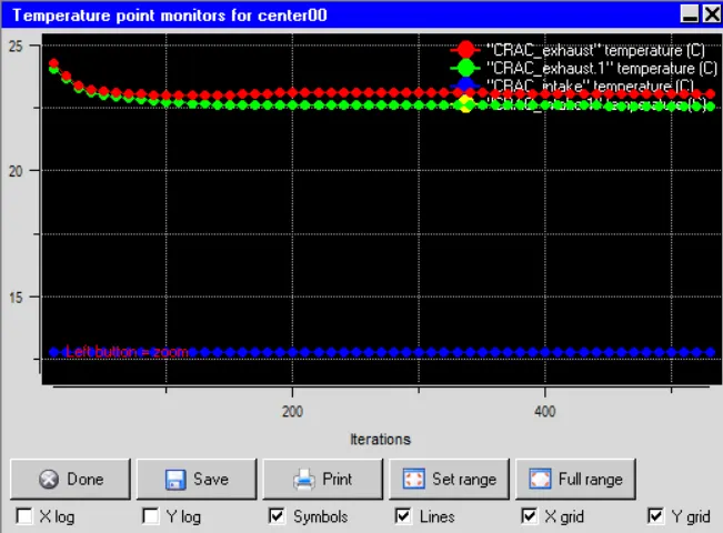
It can be seen that after 100 iterations there is no appreciable change in the recorded temperatures which indicates that the energy equation has possibly converged. According to the plot, the objects attain the following steady-state temperatures:

Results:

Temperature Contours:

• Filled colors, give a good visualization for the temperature, pressure, and mass flow rate, etc.
• The color legends are used to show the temperature contour.

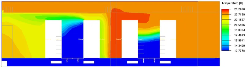
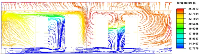
• The above contour shows the temperature behaviour inside the modeled datacentre.
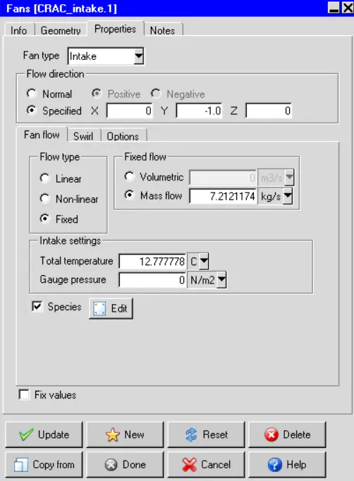
• The inlet temperature from the CRAC units is 12.78 degrees centigrade. But due to the inside temperature or the server racks temperature, the temperature hike is observed and raised up to 29 degrees centigrade.
• In the total of 4 server racks, we have given different heat flux. So that the temperature difference at the server racks has been observed.

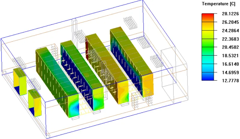
• The above picture is the Object face of some of the components we have modeled. The behaviour of the temperature of the server racks has been demonstrated with the contour colors.
• Because of the server rack, 4 is far from the tiles, the highest temperature is recorded at the one of the sides of the servers.
• Due to the difference in the heat flux of server racks, we have given 3000 Watt and 5000 watt for a couple of servers.

Velocity:

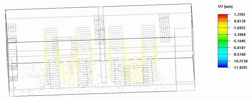
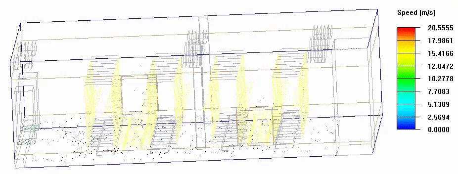
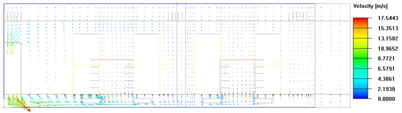
• Through CRAC units the air intake has happened and through the exhausts of CRAC warmed air is circulated and went outside.
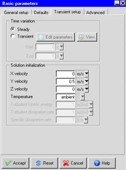
• The intake velocity of 0.5 m/s is provided in the Y-direction for the circulation of air inside the modeled data center.

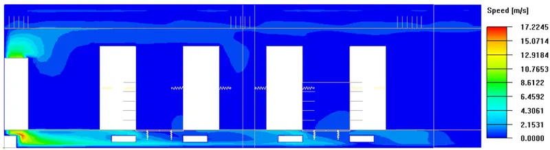
• The inlet velocity is given in the Y-direction with 0.5 m/s.
• The maximum velocity circulated and calculated as 21.3 m/s.
• The max. velocity attained at the location of CRAC unit intake, and from there the air is circulated into the entire data center with the dissipated velocity.

Vector:

Conclusion:

• The Datacentre is modeled with the macros as mentioned in the challenge. Using macros, the components like PDUs, CRACs, server racks, etc are provided.
• Using the grouping concept, all the components have been merged into particular groups.
• Using object-specific meshing parameters, the meshing of components like computer room air conditioning units (CRACs), server cabinets, power distribution units (PDUs), and perforated floor tiles have meshed to maintain the accuracy in the captured physics.
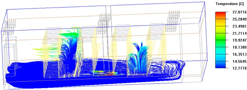
• Finally, to understand the flow of air and temperature stratification, the post-processing tools like contours, object faces, vectors, and particle traces have been used.