Week 10: Project 1 - FULL HYDRO case set up (PFI)
Aim:- To do a full hydrodynamic simulation of port fuel injection and post-process the results.
Introduction:-In the previous project, a No Hydro simulation was performed on the IC Engine. Using the same case setup, a full Hydro set up will be performed, with the tools available in Converge such as Spray and Combustion modelling. The theory related to the Full Hydro Simulation will be explained in the Case Setup under relevant headings.
Geometry:- The same geometry which was used for the "No Hydro" simulation was used for this simulation.
Case Setup:-
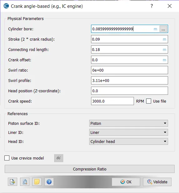
1. Application type:- Application type was set to Crank Angle-based IC engine. The values for geometry specifications such as bore dia, rpm, etc were obtained from the Engine Geometric parameters provided in the question.
2. Materials:-
-Gas Simulation:- Default values used
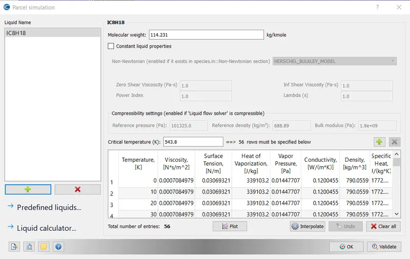
-Parcel Simulation:- When we are modelling a simulation that has fuel spray in it, the fuel spray is represented as a Lagrangian Parcel. A lagrangian-based spray model is referred to as a parcel. In this case setup, IC8H18 is the fuel spray.
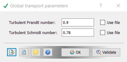
- Global Transport Parameters:- Default value retained
- Reaction Mechanism
therm.dat and mech.dat values loaded into the profile.
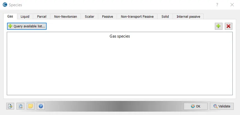
- Species
IC8H18 has been added to the 'Parcel'.
3. Simulation Parameters:-
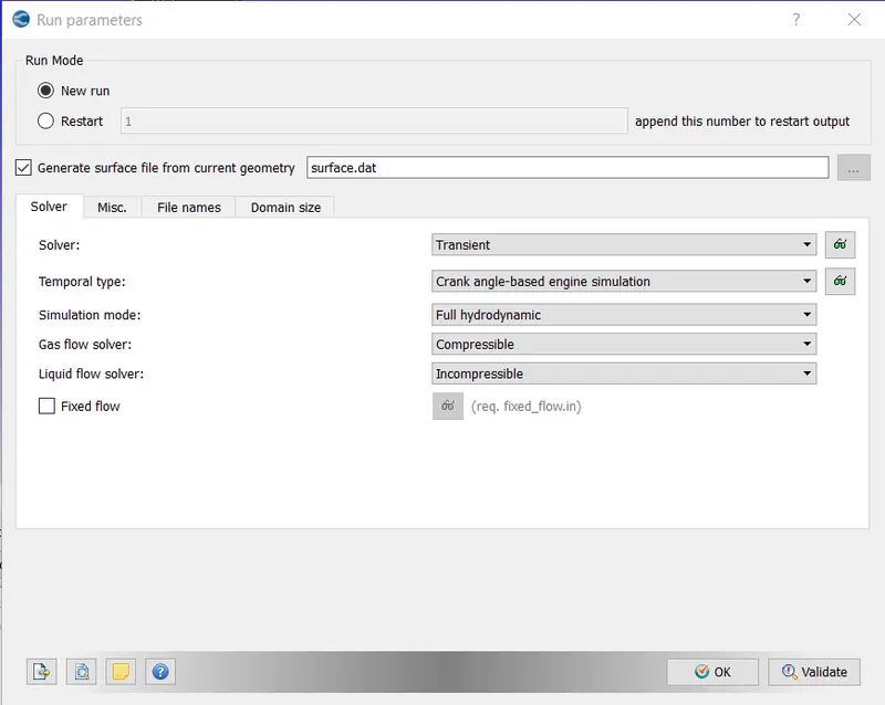
-Run Parameters:- Simulation Mode set to Full Hydrodynamic
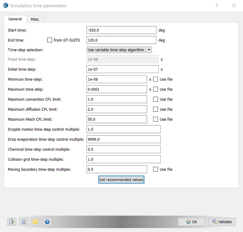
-Simulation time Parameters:-
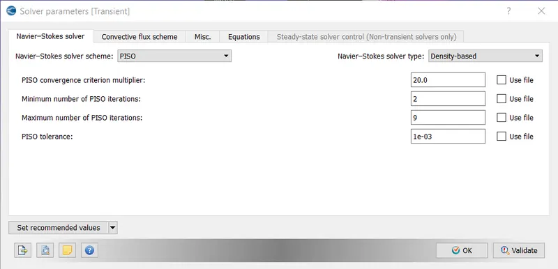
- Solver Parameters:- Default PISO scheme and Density-based solver used.
4. Regions and Events:-
A region is a collection of boundaries used to differentiate different areas in the boundary. Regions are useful for a variety of reasons
- Used to specify initial conditions by regions
- Control Flow between regions (via events)
- Output results on a region by region basis
-Apply grid control techniques by regions
-Map solutions by regions
-Specify combustion models by region
-Determine time step by region-specific CFL numbers.
Events control when the flow is permissible between regions.
In this case, set up there are four regions that have been set up, namely Cylinder region, Intake 1, Intake 2 and Exhaust regions
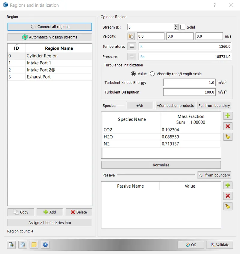
0) Cylinder region:-
- Temperature - 1360 K (Value provided in the question)
- Pressure-185731 Pa (Value provided in the question)
- Computation of Species mass concentration:- It is assumed that stoichiometric combustion of IC8H18 takes place in the combustion chamber

In the above-balanced equation, the coefficients of the products are in moles. However, CONVERGE accepts only mass fractions. Moles were converted into mass fractions with the help of an excel spreadsheet.
| Species | Moles | Molecular Weight (g/mol) | Mass (g)(Mass*Mol Weight) | Mass Fraction |
| CO2 | 8 | 44.01 | 352.08 | 0.192304403 |
| H2O | 9 | 18.01528 | 162.1375 | 0.088558734 |
| N2 | 47 | 28.0134 | 1316.63 | 0.719136864 |
| 1830.847 |
These values were inserted into species.
1) Intake Port 1:- In this port air-fuel mixture is introduced
Mass fraction of species is computed from comparable air-fuel mixture used for SI engine.
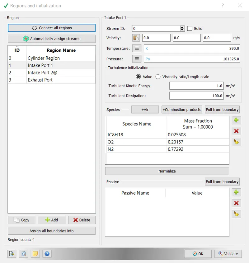
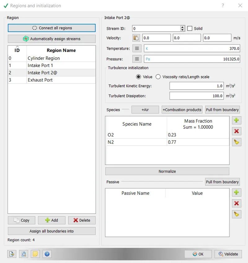
2) Intake Port 2- Air is introduced through this port. So the standard composition of sir fuel mixture is used through this port
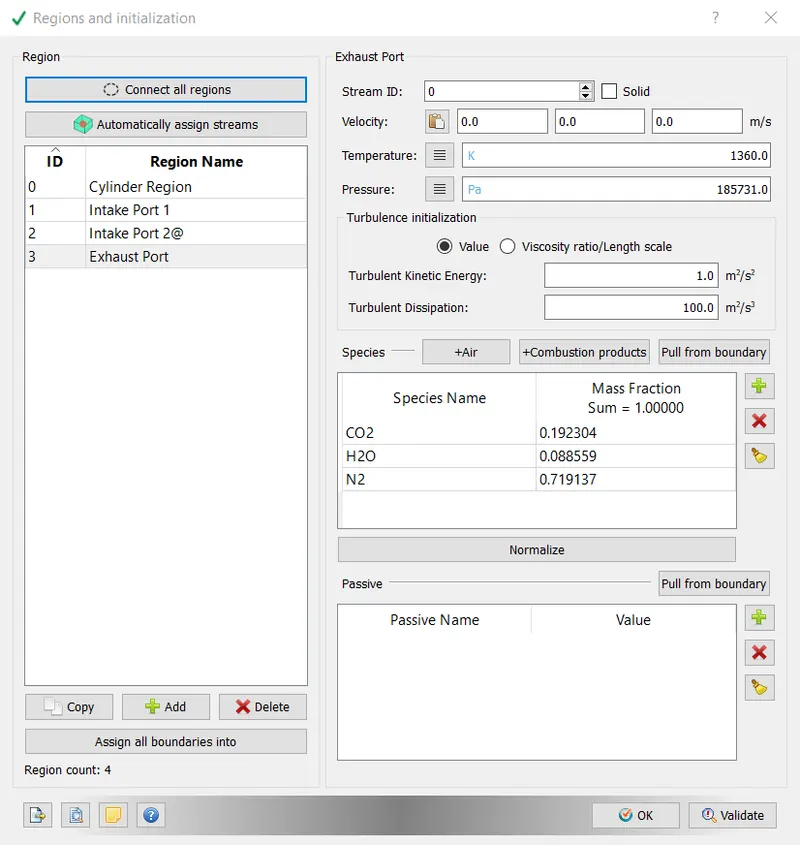
3) Exhaust Port- It is assumed that whatever is products from the combustion chamber is exhausted through the port, so the composition of products through the port is the same as that of the combustion chamber
5. Boundary Conditions:-
The component of the ICE engine was classified into different regions as shown below
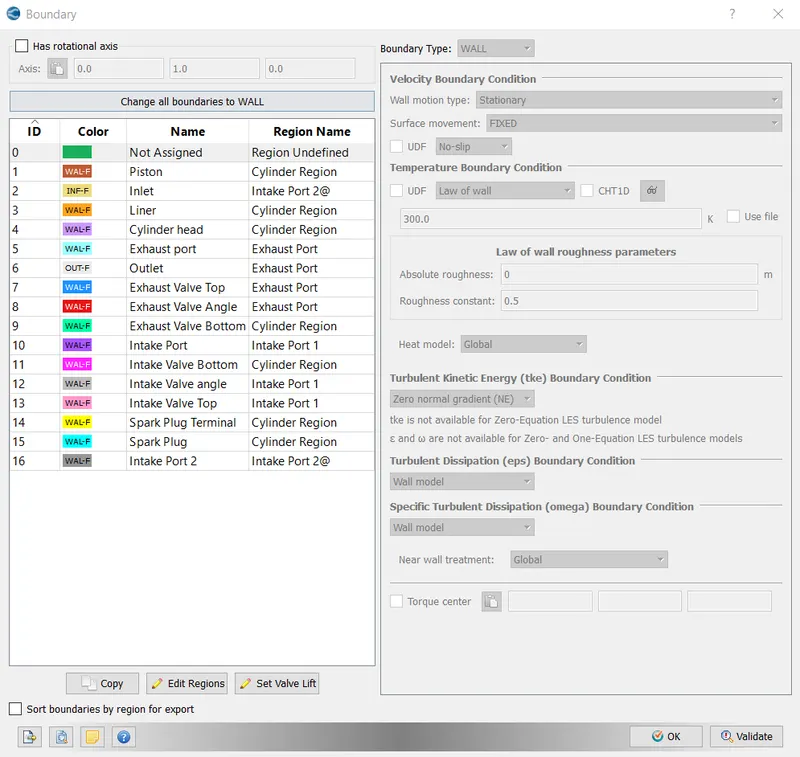
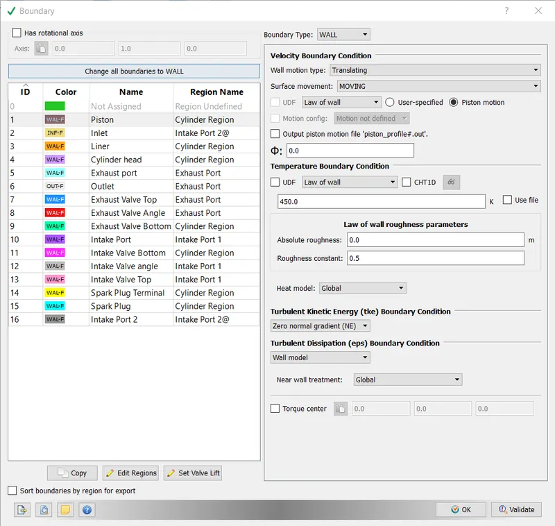
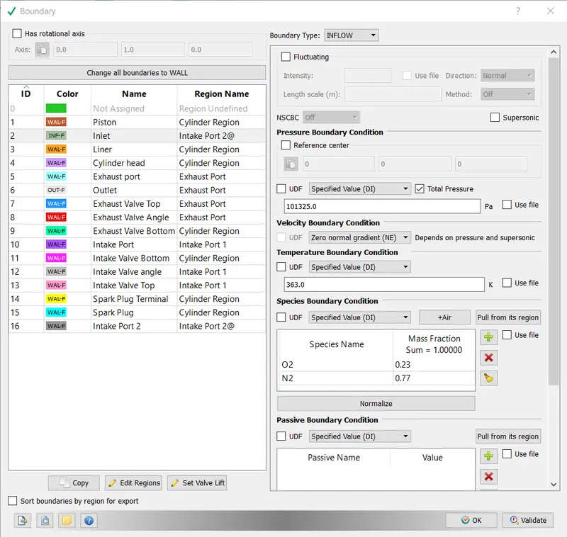
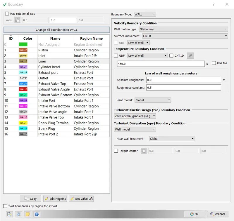
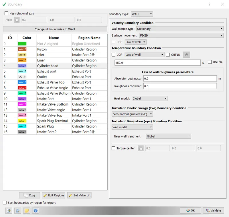
The boundary condition for each component has been set as shown below.
- Piston:- Boundary Type- Wall
- Inlet:- Boundary Type- Inflow
- Liner:- Boundary Type- Wall
- Cylinder Head:- Boundary Type- Wall
- Exhaust Port:- Boundary Type- Wall
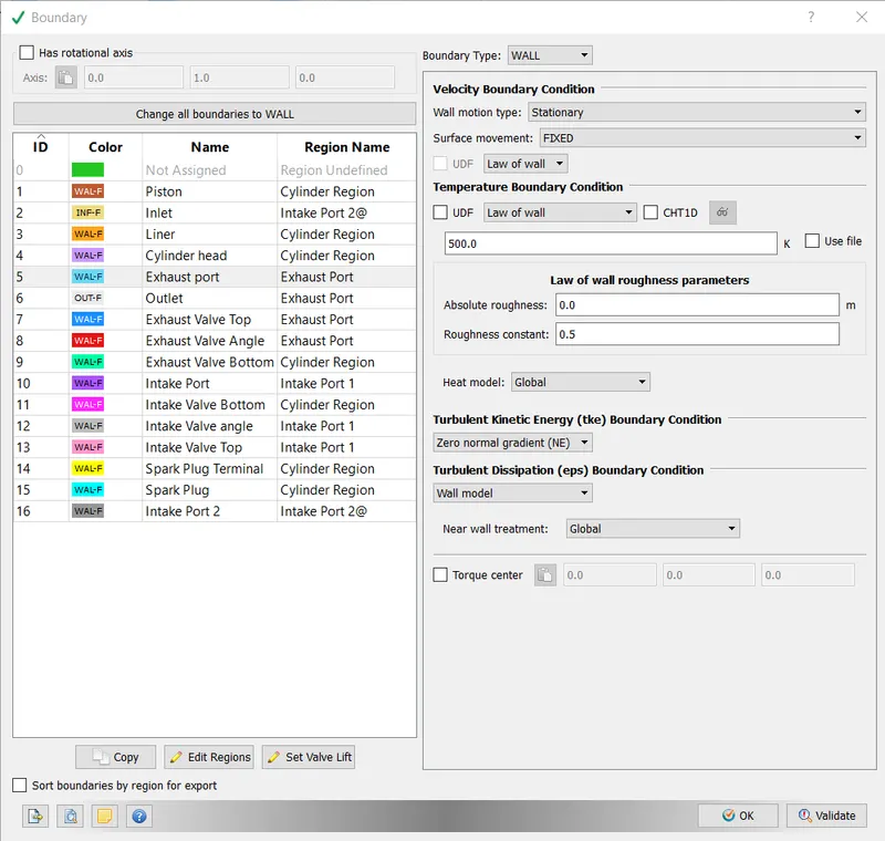
- Outlet:- Boundary Type- Outflow
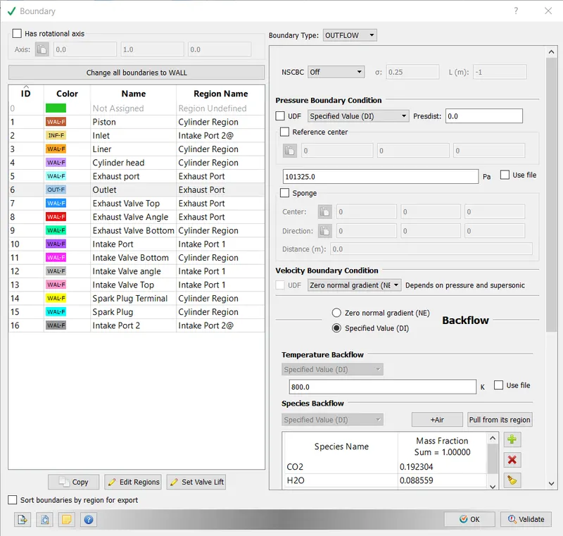
- Exhaust Valve Top:- Boundary Type- Wall, Movement as per exhaust_lift.in
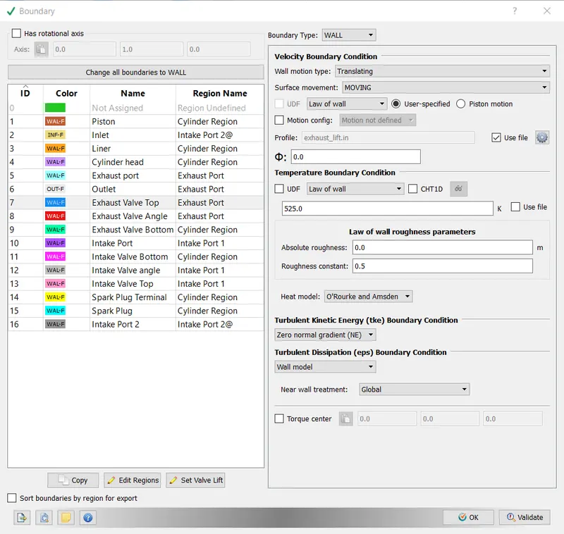
- Exhaust Valve Angle:- Boundary Type- Wall. Movement as per exhaust_lift.in
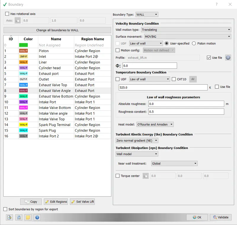
- Exhaust Valve Bottom:- Boundary Type- Wall. Movement as per exhaust_lift.in
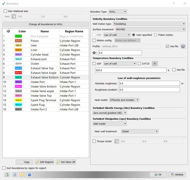
- Intake Port:- Boundary Type- Wall
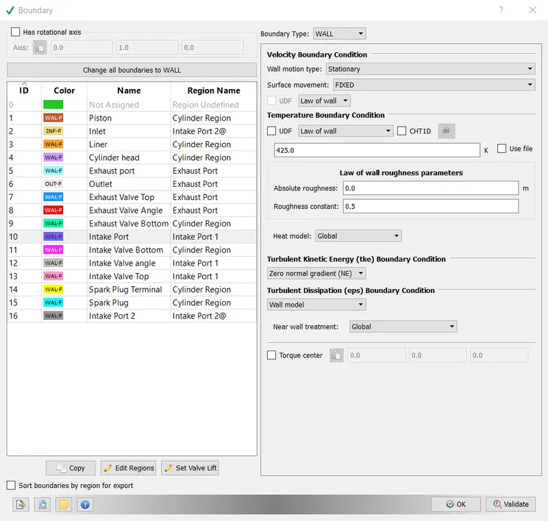
- Intake Valve Bottom:- Boundary Type- Wall. Movement as per intake_lift.in
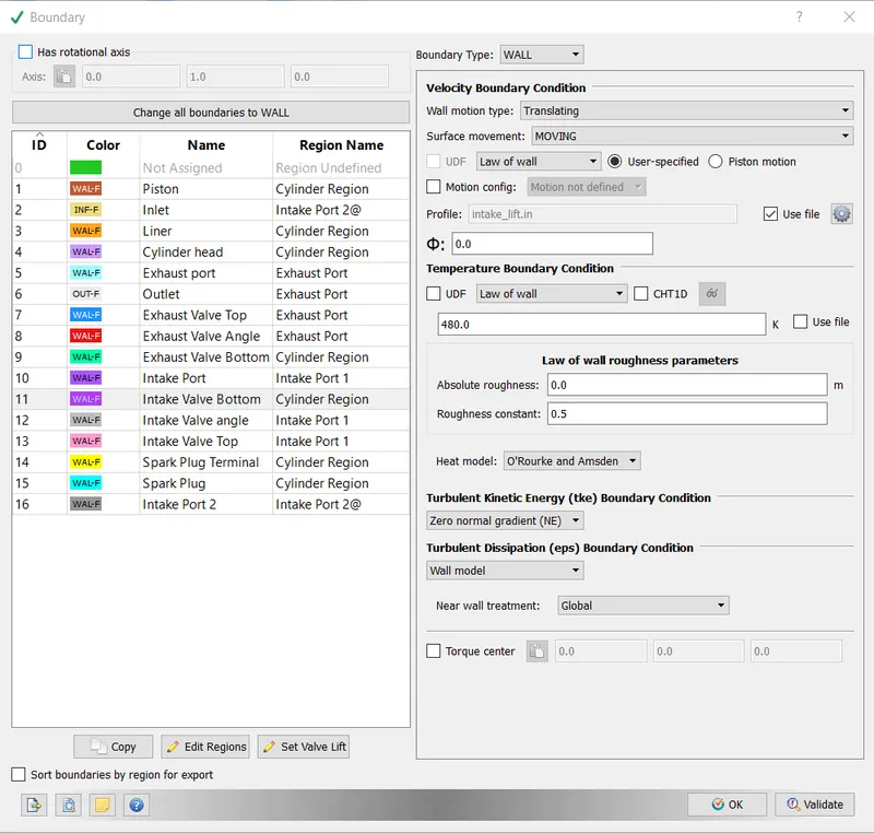
- Intake Valve Angle:- Boundary Type- Wall. Movement as per intake_lift.in
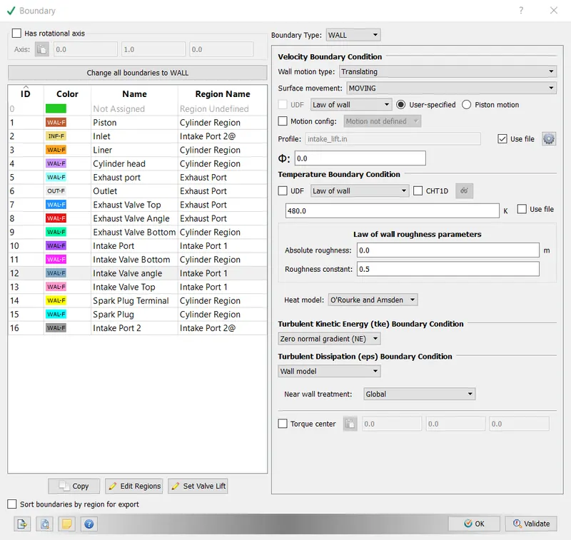
- Intake Valve Top:- Boundary Type- Wall
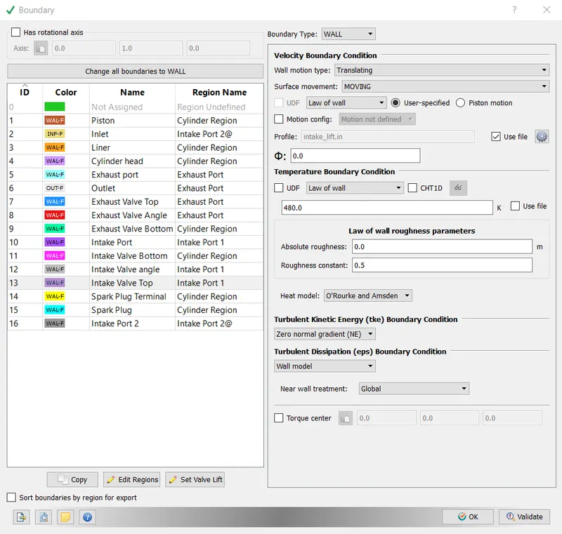
- Spark Plug Terminal:- Boundary Type- Wall
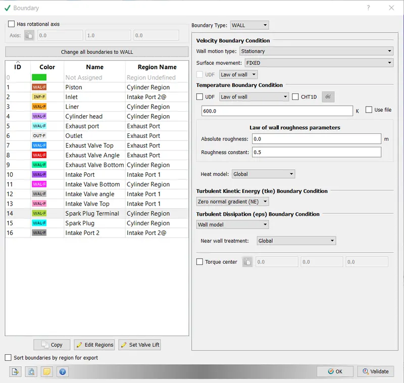
- Spark Plug:- Boundary Type- Wall
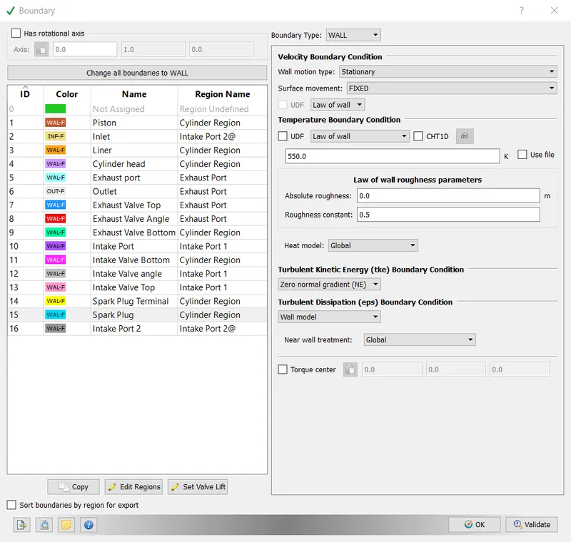
- Intake Port 2:- Boundary Type- Wall
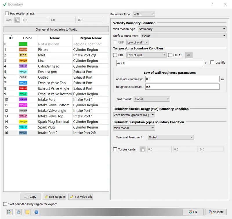
Physical Modelling:-
-Spray Modelling:-
Spray modelling is required because solving fluid flow equations describing spray motion directly is not computationally feasible. So a modelling approach is adopted which captures the physics of spray motion.
For liquid sprays, Converge uses a Langrangian solver to model discrete parcels and the Eulerian solver to model the continuous fluid domain. Heat, momentum and Mass transfer occur between the discrete and continuous phases via source terms in the transport equation.
Converge introduces parcels (collection of drops) into the domain at the injector. Each parcel represents a group of identical drops (same, radius, velocity, temperature). CONVERGE solves for radius, velocity on a per parcel basis.
Parcel undergo several Physical processes.
-Primary Breakup
-Secondary Breakup
-Drop Drag
-Collision and coalescence
-Turbulent dispersion
-Evaporation
When fuel is injected, the liquid particles interact with the surrounding air. This interaction causes the creation of drag forces that results in the propagation of disturbances. If the liquid particle is large enough it breaks into smaller particles which then break up into even smaller particles (Primary and secondary breakup). When the smaller secondary particles interact with ambient air, they undergo one or more of the other physical phenomena, namely drop drag, collision and coalescence, Turbulent dispersion and Evaporation.
For the purpose of the Full Hydro Case simulation, the following approach was adopted.
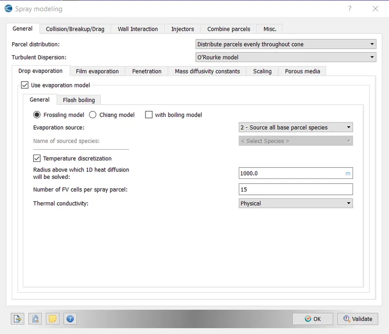
- General Setup
i) Parcel Distribution- Distribute Parcels evenly throughout the cone
ii) Turbulent Dispersion - O Rourke Model (For a gasoline engine, O Rourke model gives better results)
iii) Evaporation Model enabled
iv) Frossling model selected
v) Evaporation source:- Source all base parcel species selected (This implies that IC8H18 (liquid) converted to IC8H18 (gas)
vi) Temperature Discretization enabled
vii) Radius above which 1 D heat equation will be solved = 1000 m
viii) No of FV cell per spray parcel =15
ix) Thermal conductivity- Physical
- Collision Break up and modelling
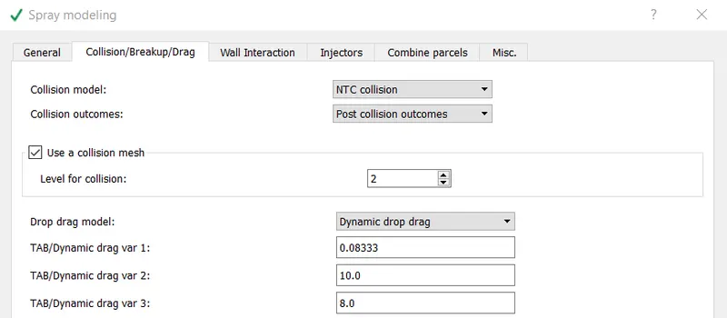
i) Collision model:- NTC collision used
ii) Collision outcomes:- Post-collision outcomes
iii) Use a collision mesh option enables
iv) Drop drag model- Dynamic drop drag
v) Dynamic drag values set as shown below
- Wall Interaction:-
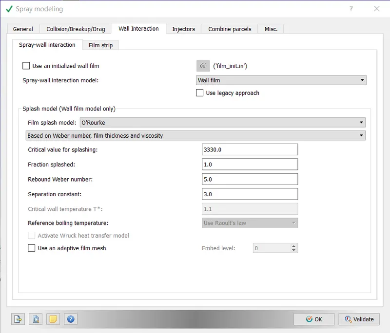
For Wall Interaction, default values have been retained
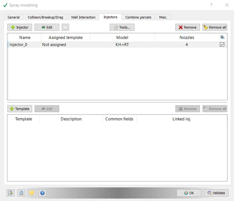
- Injector Modelling
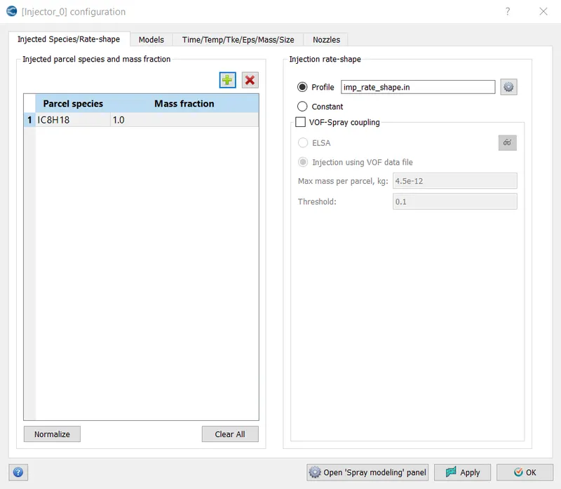
i) Injected Species:- Parcel Species set to IC8H18 with mass fraction set to 1.0. An injection rate shape profile was imported.
- Models
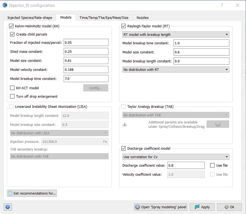
Kelvin- Helmholtz model and Rayleigh- Taylor Model was selected as these are the commonly used models for solid cone sprays. The default constants were retained. The discharge coefficient was set to 0.8.
The default constants control how the breakup of the liquid particles. The stability equation governs the process however do not capture the finer details. The constants govern how long it takes for the breakup and the size of the child droplets.
-Injector configuration
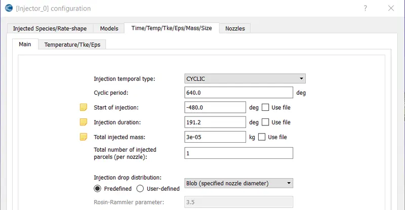
i) Injection temporal type - CYCLIC
ii) Cycle period - 640
ii) Start of Injection= -480 degree (Given)
ii) Injection duration = 191.2 degree (Given)
iii) Total injected mass is calculated as shown below
Fuel flow rate = 7.5 e-4 kg/s
Engine RPM=3000
Engine RPS = 3000/60 =50 rps
Engine Degree Per Second= 50 * 360= 18000
Time per degree= 1/18000= 0.00005555555
Time for 720 degrees= 0.00005555555*720 = 0.04 seconds
Fuel flow rate= 7.5 e-4*0.04=3 e-05 kg/sec
-Nozzles
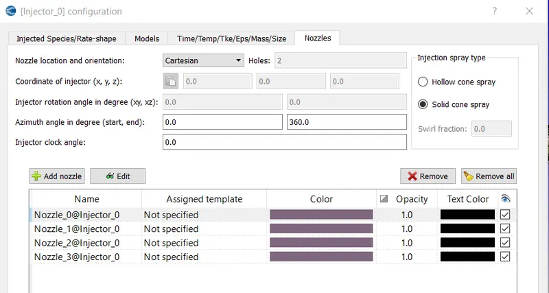
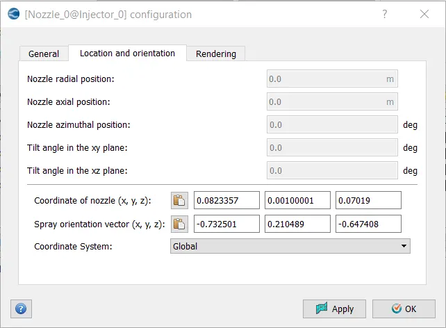
i) Nozzle Location and orientation -Cartesian
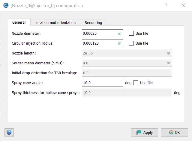
ii) Nozzle diameter=0.00025m (Given)
iii)Circular Injection -0.000123m (Injection dia= Nozzle radius)
iv)Nozzle location set as per provided location
v) Spray Cone Angle -10 degree (Usually between 10-15 degrees)
Computation of Maximum Injection pressure:-
Peak Injection Pressure = 4.29908 (bar)
Peak Injection Velocity New = 29.7017 (m/s)
Validation of Nozzle Locations. To ensure the newly created nozzles were inside the computational domain, the Tools-Validate Nozzle location was selected upon which the below item was displayed.
-Combustion Modelling:-
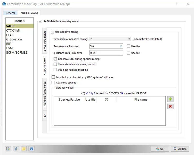
Combustion facilitates energy transfer in an engine. The Combustion model which is used for IC engines is the SAGE detailed Chemistry Solver. SAGE solver is the most predictive and accurate way to model combustion. It models ignition and laminar flame propagation quite accurately.
The SAGE model uses local conditions to calculate reaction rates based on the principle of chemical kinetics. it solves detailed chemical kinetics during combustion and determines kinetically limited phenomena such as engine knock and emissions. It reads in a reaction model in CHEMKIN format and solves ODE's to determine reaction rate. It also computes the rate of change of species concentration using the Arrhenius law. At each time step, the Chemistry solver calculates new species mass fraction immediately prior to solving the transport equation. System of elementary reactions solved using CODES.
Solving SAGE equations is a computationally slow process. In order to decrease the computational time, CONVERGE includes the following options
- Increase minimum cell temperature and minimum HC species mole fraction to reduce the number of cells in which combustion calculations are performed
- Use Start time and end time to limit SAGE to specific time intervals
-Limit SAGE to specific regions.
- Set resolve option to Only resolve if temperature changes by a specified value.
- Use analytical Jacobian to pass analytically calculated Jacobian to the solver.
- Multizone models are used to reduce the number of SAGE calculations.
For the purpose of the simulation, the case was set up as shown below
The SAGE detailed chemistry solver parameters were set as follows.
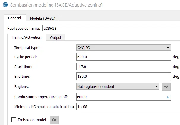
The General setting values were set as shown below.
The combustion was set to start a few crank angles before ignition. The end time for combustion was set considering the opening of the exhaust valve.
- Spark Plug modelling
In a typical spark discharge, the Voltage rises between two electrodes until there is a breakdown in the spark gap. The first stage is called the breakdown phase in which the mixture between the electrodes is ionized into plasma. The breakdown phase is followed by the arc phase in which thin cylindrical plasma expands largely due to heat conduction and diffusion. The arc phase is followed by the glow discharge phase, energy storage device will dump its energy into discharge circuits. Time scales in the breakdown phase are significantly lower than the arc/glow phase. In converge simulation, we specify two phases that briefly overlap.
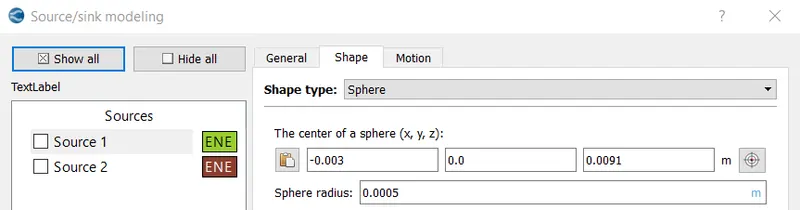
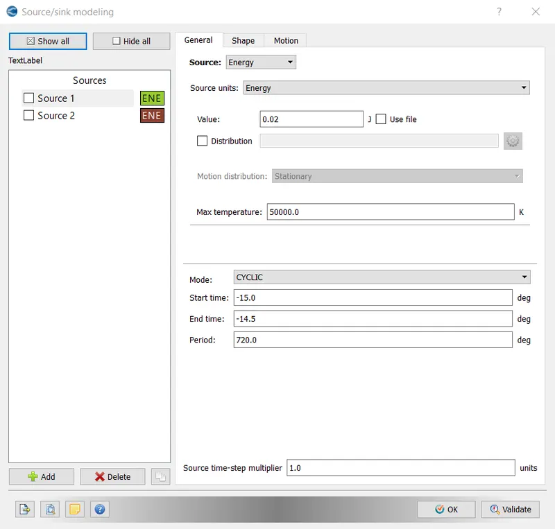
In order to model the operation of the Spark Plug, the source/sink modelling option was enabled. Two spherical sources were created with a radius of 0.5mm. The centre of the sphere location was taken from the spark location
- Shape
The general values were set as shown below. The spark start and end times were set from the values provided.
7. Grid control:-
CONVERGE uses a number of tools for controlling grid size during a simulation. Fixed embedding refines a grid at specified locations and times. Grid scaling coarsens or refines the base grid size. Adaptive Mesh Refinement automatically changes the grid based on fluctuating and moving conditions.
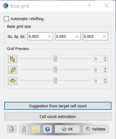
- Base grid size was set to 0.005
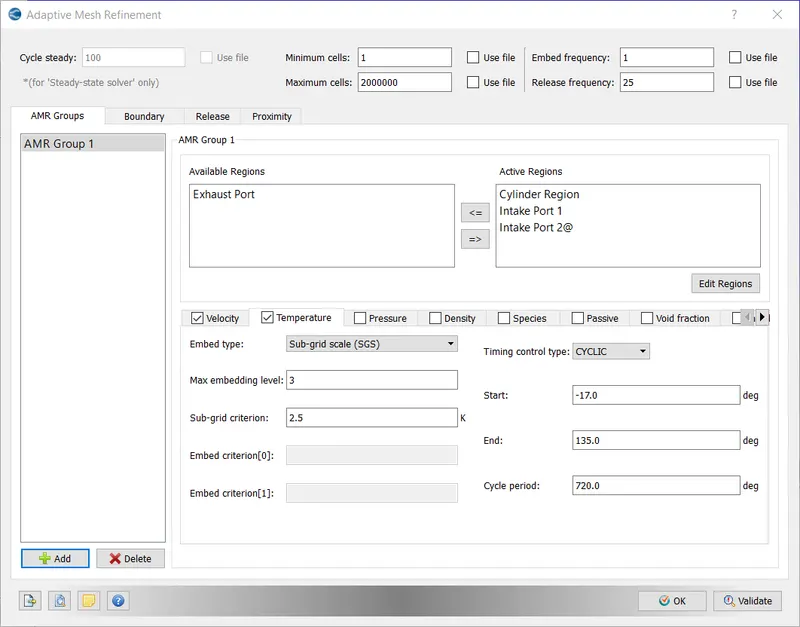
- Adaptive Mesh Refinement
Adaptive mesh refinement increases grid resolution based on curvatures (second derivatives in-field variables). It can be permanent or activated at specific times. It is can be activated on a region by region basis. It can be activated for both scalar and vector fields.
CONVERGE calculates the Subgrid Scalar (SGS) field as
where `phi''= sub grid scalar field
'phi'= actual field
'barphi'= resolved field
CONVERGE uses truncated infinite series to approximate subgrid scalar field for any scalar.
where 'dx_k' is the spacing for a given rectangular cell.
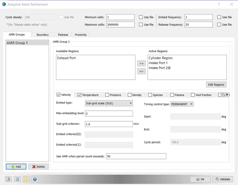
For the full hydro set up two types of AMR is used
1. Velocity
The maximum no of embedding levels is 3
SGS criterion is 1m/s
Whenever the curvatures exceed 1m/s, the regions would be automatically refined.
The timing control type is Permanent.
2. Temperature.
Max embedding level 3.
SGS criterion 2.5 K.Whenever the curvatures exceed 2.5K, the regions would be automatically refined.
Timing control type- Cyclic
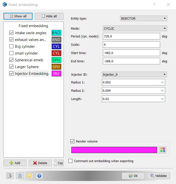
-Fixed Embedding
Fixed embedding allows to locally refine the mesh in the domain where a finer detail is critical to the accuracy of the solution.
An embedding scale is specified which indicates how CONVERGE will refine the grid in that location
dx_embed= dx_base/(2^(embed scale))
For the Full Hydro setup Fixed embedding was used at the below location
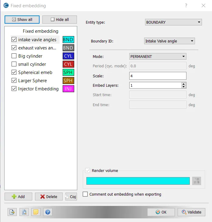
1. Intake Valve angles:-
Entity type- Boundary
Mode - Permanent
Embed Scale = 4
Grid size at refined locations = 0.005/2^4 =0.0003125
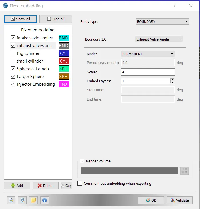
2. Exhaust Valve angles
Entity type- Boundary
Mode - Permanent
Embed Scale = 4
Grid size at refined locations = 0.005/2^4 =0.0003125
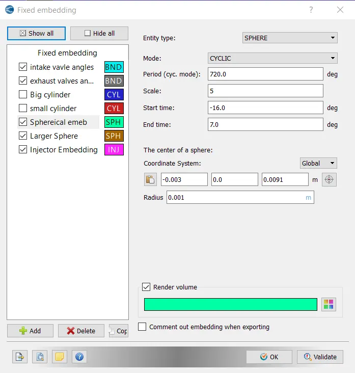
3. Spark Plug
Entity type- Sphere
Mode - Cyclic
Embed Scale = 5
Grid size at refined locations = 0.005/2^5=0.00015625
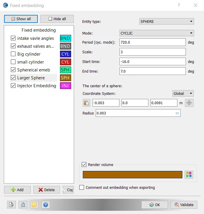
4. Large Spherical
Entity type- Sphere
Mode - Cyclic
Embed Scale = 3
Grid size at refined locations = 0.005/2^3=0.000625
5. Injector
8. Results:-
a) Compression Ratio:
In a reciprocating engine, the piston oscillates between the Top dead center and the bottom dead center. These correspond to the minimum and maximum values respectively. The ratio between these two volumes is known as the compression ratio.
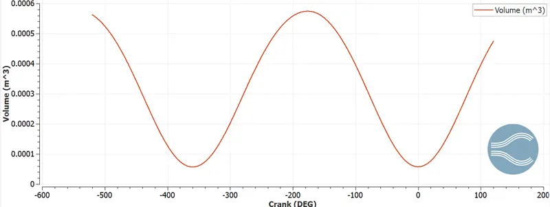
From the above graph we, note that
Maximum Cylinder Volume = 5.74186 X10^-4 m^3
Minimum Cylinder Volume =5.73996 X 10^-5 m^3
Compression ratio=(5.74186 X10^-4)/(5.73996 X 10^-5)=10
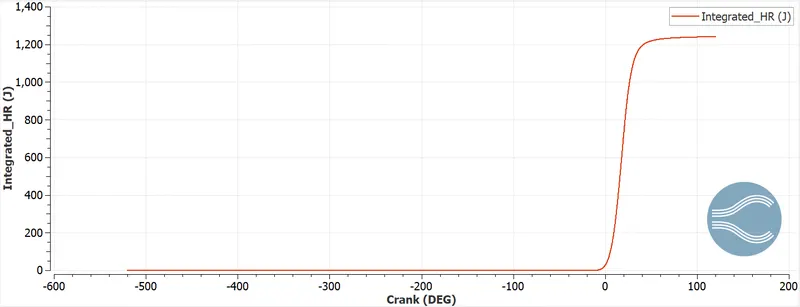
b)Calculating the Combustion efficiency of the Engine
Combustion efficiency is defined as the energy released by the burnt fuel to the theoretical energy content of the fuel

Integrated Heat Release Rate= 1241.15 J
m_f= Mass of Fuel, kg/sec= 3x10^-5 kg
LHV= 43.4 MJ/kg

c) Power & Torque Consumption
Power is defined as the rate of doing work.
Work = 468.646 Nm
Duration= 120.11+120.09= 240.2 degree
RPM=3000
RPS= 3000/60=50
1 revolution/sec= 360 degrees
50 revolution/sec= 50 *360= 18000 degree
Time (sec)= 240.2/18000=0.0133444 sec
Power = Work/sec= 468.646/0.0133444 =35119.301 J/sec
Power = 35.119 KW
Torque
The equation for Power is given below
N= revolution per sec
T= Torque
Re arranging for Torque
'T=(P)/(2piN)'
= 35.119*1000/(2*pi*50)
=111.878 Nm
The PV diagram for the engine is given below. Area under the PV diagram signifies the work done.
d) Need for Wall Heat Transfer model
Heat loss through the cylinder walls has a detrimental impact on the performance of the engine. Some of the undesirable effects include reduction in volumetric efficiency, incomplete combustion etc. The description of heat transfer in an ICE is a challenging task, considering the different systems (intake and exhaust ports, coolant circuit, lubricant oil subsystem), the different heat transfer mechanisms (convection, conduction and radiation), and the rapid and unsteady changes that take place inside the cylinder
So there is a need to accurately model this phenomenon. Due to the complexity involved in a mathematical solution, there is a need to adopt suitable modelling
e) Why we cannot use CFD to predict wall temperature?
(CFD) can provide precise and instantaneous information about the flow within the engine (temperature, pressure, velocity distributions), but require temperature boundary conditions for the engine walls, which are typically assumed as being constant throughout the engine cycle. This will affect the combustion process, thus leading to inaccurate results Imposing appropriate wall temperature boundary conditions is not an easy task, and may require some iterative process. However, such calculations with a given surface temperature are not sufficient when the focus is on analyzing the heat transfer within the engine. The heat flux and gas properties of the CFD are used as boundary conditions for the heat conduction calculation of the solid regions.
f) Significance of CA10, CA50 and CA90
The CA10, CA50 and CA90 are defined as positions of the crank angle at which cumulative heat release rate reaches 10%, 50 % and 90%. The physical significance of CA10 is that it is used to signify the start of ignition in an engine, while CA 50 signifies the end of pre-mixed combustion and the start of diffusion combustion of fuel used in the engine. The greater the difference between CA10 and CA50, the higher is the duration of combustion and vice versa.
g) Other Plots
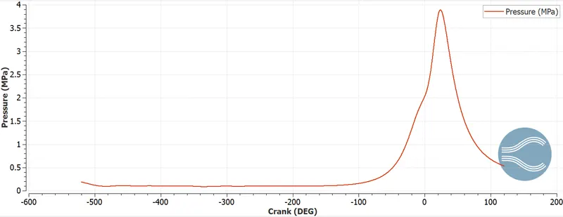
1) Cylinder Pressure:- The plot for cylinder pressure as a function of crank angle is given below. It is noted that the cylinder pressure peaks during the compression stroke (compression occurs between -120 degrees to 120 degrees).
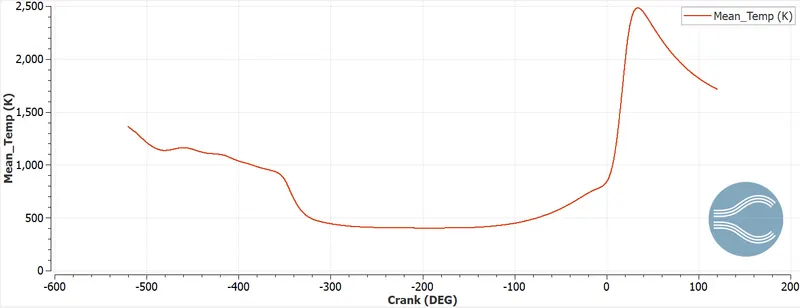
2) Mean Temperature:- The plot for peak mean temperature in the cylinder region as a function of crank angle is given below. It is noted that peaks of temperature and pressure coincide and occur during the combustion stroke.
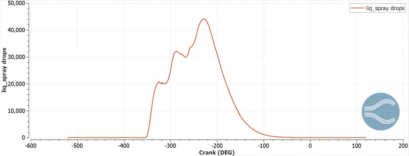
3)Liq Spray Drops (Cylinder region):-It is noted that the maximum liquid droplets present in the cylinder are around 450000. This decreases after some time due to evaporation and combustion. Eventually, this drops to a nearly zero value. From this, we infer that combustion is nearly complete in the cylinder.
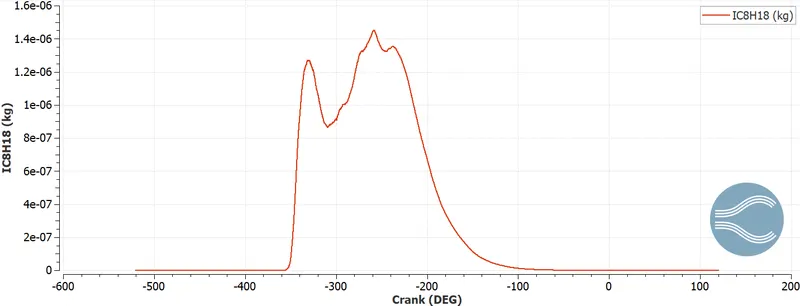
A similar trend is observed for IC8H18, The mass peaks at a certain crank angle after which it decreases due to evaporation and combustion and reduces to a near-zero value. This indicates that the combustion process does not leave any unburnt fuel in the engine.
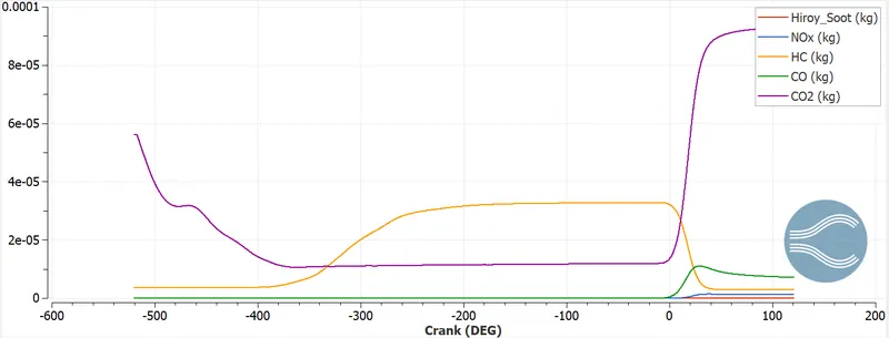
4) Emissions:- The emission quantities of various gases as a function of crank angles are presented below.
h)Animations:
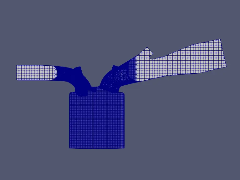
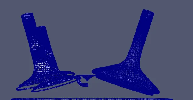
i) Meshing:- From the below plots we can see that regions of the mesh get refined in accordance with Adaptive Mesh refinement and Fixed embedding criteria that were set during the case setup stage
- Overall Mesh
Valves
ii) Temperature:-
In the above animation, we can observe the variation of temperature over the course of the four-stroke combustion process in the IC engine. As expected, during the combustion process, the temperature in the cylinder reaches the maximum. During the exhaust stroke, the temperature in the exhaust port/valves registers an increase.
iii) Spray Modelling
The fuel injection in the engine during the four-stroke combustion process is captured in the below animation. The movement of spray particles through intake ports and to through the cylinder is observed.
9. Conclusion:-
In this project, a detailed simulation of the IC engine has been carried out. In the case setup, spray and combustion modelling was set up. Movement of piston, intake and exhaust valves were created using regions and events. Mesh refinement techniques such as AMR and Fixed embedding were adopted to obtain finer results.
After simulation and post-processing, engine performance parameters such as compression ratio, power and torque were computed and are listed below
Compression Ration=10
Power = 35.119 Kw
Torque= 111.8 Nm
Apart from this, other aspects such as cylinder mean temperature and pressure, liquid particles and emissions were studied as a function of a crank angle. Also, animations for temperature and spray modelling were examined,