Week 2 - Flow over a Cylinder.
AIM:- Vortex shedding simulation over a cylinder in laminar flow.
Objective:-
- Simulate the flow with the steady and unsteady case and calculate the strouhal number for Re=100
- To calculate the co efficient of drag and lift over a cylinder by setting the Reynolds number(Re) to 10,100,1000,10000 & 100000.(Run with steady slover)
Introduction:-
Vortex shedding
Vortex shedding is an oscillating flow that takes place when a fluid such as air or water flows past a bluff(as opposed streamline) body at certain velocities, depending on the size and shape of the body. In this flow, vortices are created at the back of the body and detach periodically from either side of the body forming a Von karman vortex street. The fluid flow past the object creates alternating low-pressure vortices on the downstream side of the object. The object will tend to move toward the low-pressure zone.
If the bluff structure is not mounted rigidly and frequency of vortex shedding matches the resonance frequency of the structure, then the structure can begin to resonate, vibrating with harmonic oscillations driven the energy of the flow. This vibration is the cause for overhead power line wires humming in the wind, and for the fluttering of automobile whip radio antennas at some speed.
Flow over a cylinder is one of the basic simulation in the CFD domain and till this date the research is still going on to study the unsteady behaviour caused by the flow. The flow over cylinders is very complex and periodic flow pattern are seen at lower reynolds number and after achieving critical reynolds number value, the flow gets change in the wake region and this wake formation can be studied using literature of von-karman vortex street. Considering any other obje t compared to cylinder most of them cause boundary layer detachment due to the effect of geometry features like sharp edges but in the case of the cylinder this point of separation is very complex and depend upon nature of upstream boundary layer and other flow parameters.
The vortex induced vibration is one the key aspect which may lead to study of vortex shedding in real life applications such as bridges,aircraft control surfaces,heat exchanger and many others. The vibration caused by vortex phenomenon due to flow dynamics is need to be studied for the design and development of flow dynamics is need to be studied for the design and development of product at very good scale. The design and development of product at very good scale. The strouhal number is also used with other number in axial flow turbine to determine the frequency of the blades over the flow period.
Reynolds number(Re):-
Reynolds number for a flow is a measure of the ratio to inertial to viscous force in the flow of a fluid around a body.
Re=(rho*v*d)/(Dynamic viscosity)
The range of Re values will vary with size and shape of the body from whch the eddies are being shed, as well as with the kinematic viscosity of the fluid. over a large Red range(47<Red<105, for circular cylinder; refernce length is d: diameter of the circular cylinder) eddies are shed continuously from each side of the circle boundary, forming rows of vortices in its wake. The alternation leads to the core of a vortex in one row being opposite the point midway between two vortex cores in other row, giving rise to the distinctive pattern shown in the picture. Ultimately, the energy of the vortices is consumed by viscosity as they move further downstream and the regular pattern disappears.
Strouhal number(St):-
Strouhal number is a dimensionless number describing oscillating flow mechanisms.
The Strouhal number is often given as
St=f*D/U
where, f is the frequency of vortex shedding
D is the diameter of the cylinder
U is the flow velocity.
Co-efficient of drag(Cd):-
In fluid dynamics, the drag coefficient is a dimensionless quantity that is used to quantify the darg or resistance of an object in a fluid environment, such as air or water. It is used in the drag equation in which a lower drag coefficient indicates the object will have a less aerodyanmic or hydrodynamic drag. The drag coefficient is always associated with a particular surface area.
The drag coefficient of any object comprises the effects of the two basic contributors to fluid dynamic drag: skin friciton and form drag. The drag coefficient of a lifting airfoil or hydrofoil also includes the effects of lift-induced drag. The drag coefficient of a complete structure such as aircraft also includes the effects of interfernce drag.
The drag coefficent is defined as

where, Fd is the drag force,
ρ is the mass density of the fluid
u is the flow speed of the object relative to the fluid
A is the reference area
Co-efficient of lift(CL):-
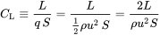
The lift coefficient(CL) is a dimesionless coefficient that relates the lift generated by a lifting body to the fluid density around the body, the fluid velocity and an associated reference area. A lifting body is a foil or a complete foil-bearing body such as fixed-wing aircraft. CL is a function of the angle of the body to the flow, its reynolds number and its mach number. The section lift coefficient CL refers to the dynamic lift charcteristics of a two-dimensional foil section, with the reference are replaced by the foil chord.
 ,
,
Where, L is the lift force,
S is the relevant surface area
q is the fluid dynamic pressure
Geometry:
A plate with the dimension of 20*60m is created using spaceclaim.
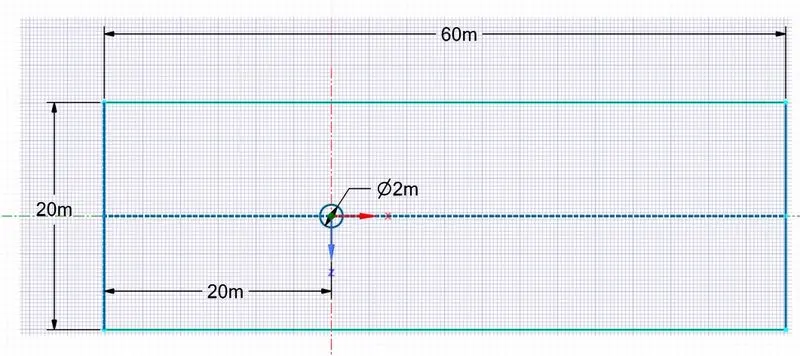
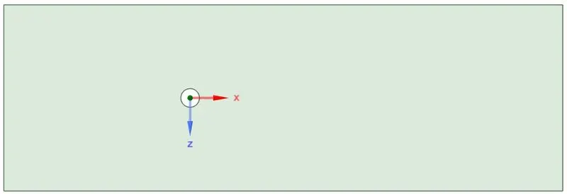
Now, we want to simulate effect of fluid flow over cylinder, select the circle and delete it.
Meshing:
- Select the edges of geometry and name inlet, outlet, wall and symmetry.
- Now select the body and got mesh and click on generate mesh with mesh size 0.m To ensure triangular mesh, go to mesh>insert>triangular mesh
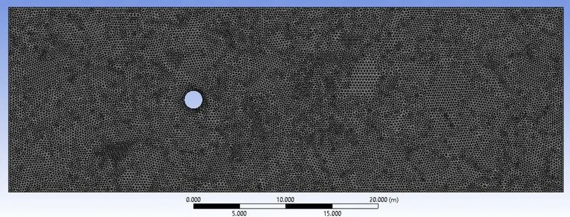
- After generating mesh, it is seen that size of circle looks distorted. Go to mesh>sizing>select circular edge>definition>type>no. of division>36
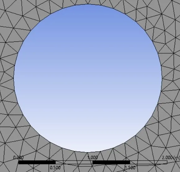
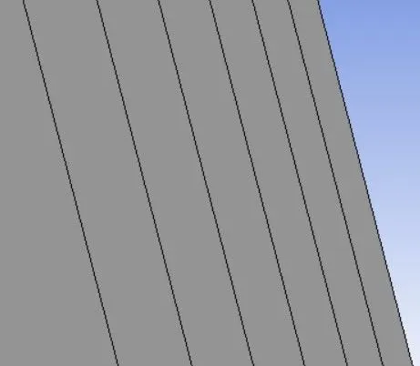
- To capture better results near cylinder wall, go to mesh>inflation>select the body and edge>inflation option:1st layer thickness>1st layer height:5e-3>maximum layer:6
Solving:
- Select laminar flow inside the viscous model.
- As we wanted to customize material property for simulation , go to materials>fluent database>select the material(air)>copy it > rename the name of the material
PART-1:-
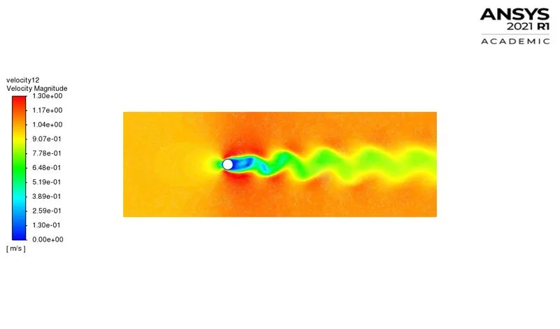
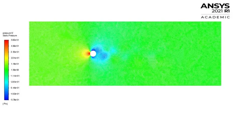
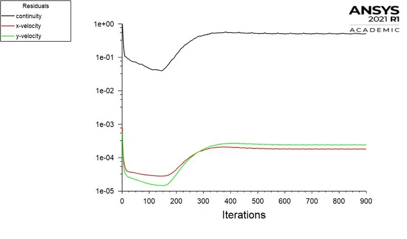
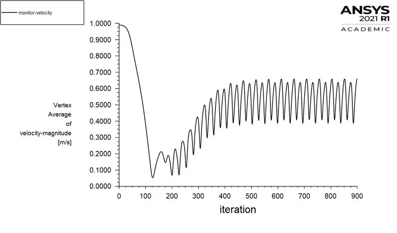
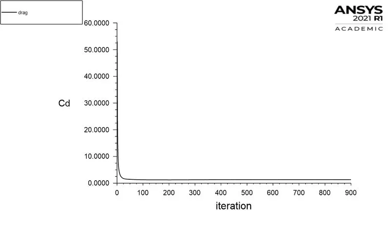
- Simulation with the steady-state solver, Dynamic viscosity=0.02kg/m.s and Re=100
A steady state solver with the laminar viscous model has been used to simulate the problem. The SIMPLE scheme with the least square cell-based system for gradients is used. Pressure and momentum interpolation schemes were chosen as second- order upwind. The B.C at inlet velocity is 1m/s. At outlet , pressure-outlet conditon is used with gauge pressure equals to zero. At the walls the no-slip condition is given and the bottom nd top boundaries were treated with symmetry B.C
Reference values:
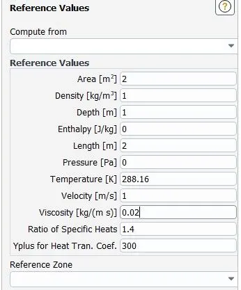
The results are given below.
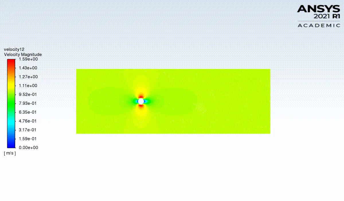
Velocity Contour:
Pressure Contour:
Residual plot:
Vertex average velocity plot:
Coefficient of drag plot:
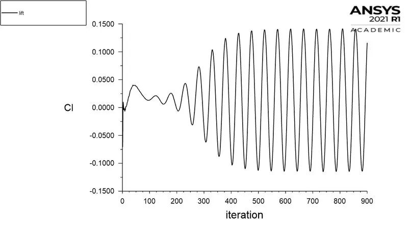
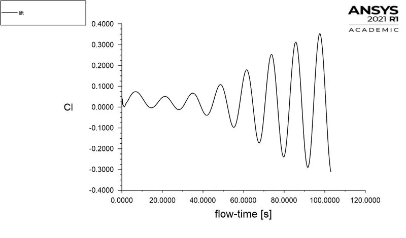
Coefficient of lift plot:
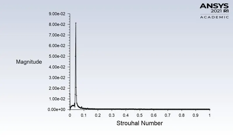
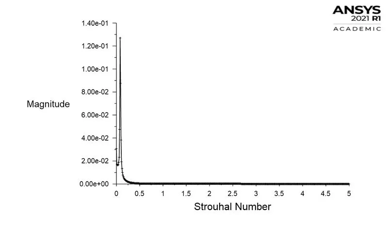
Strouhal number plot:
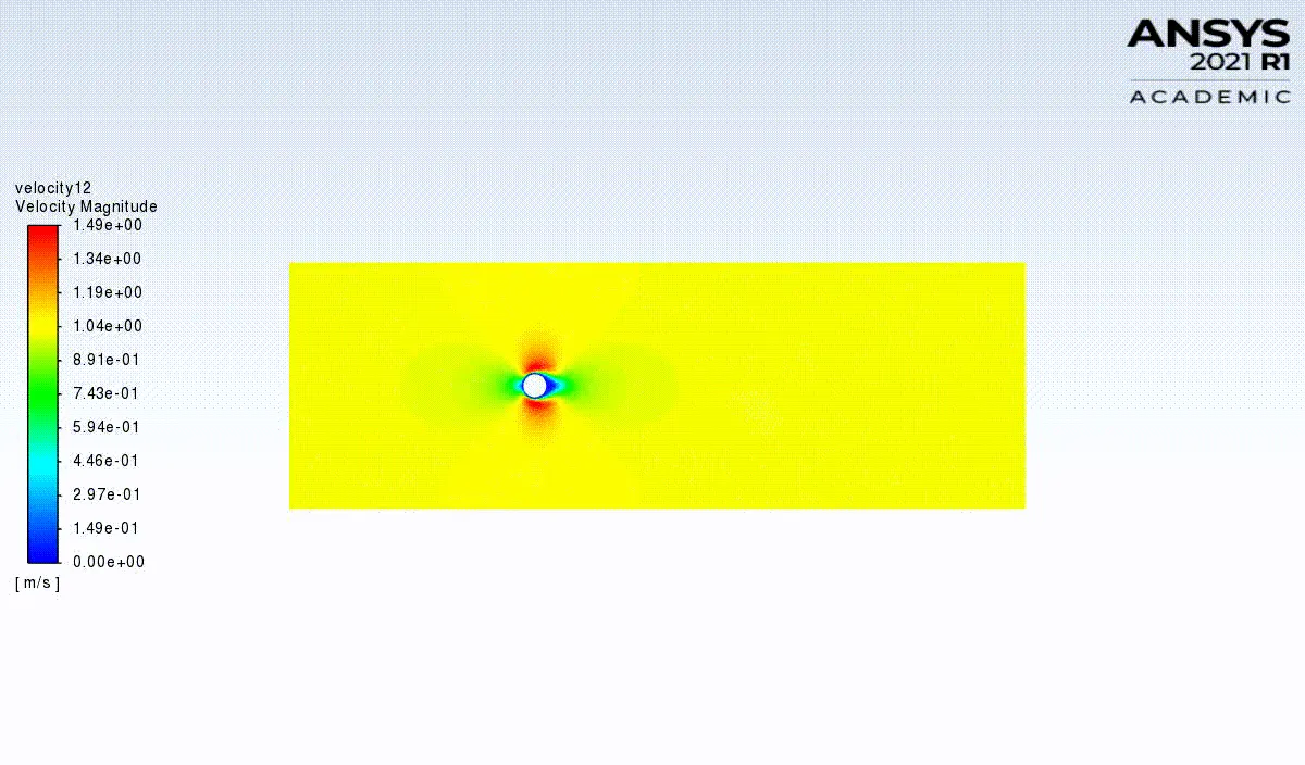
Solution animation:
b. Simulation with the unsteady-state(transient) solver, Dynamic viscosity=0.02kg/m.s and Re=100
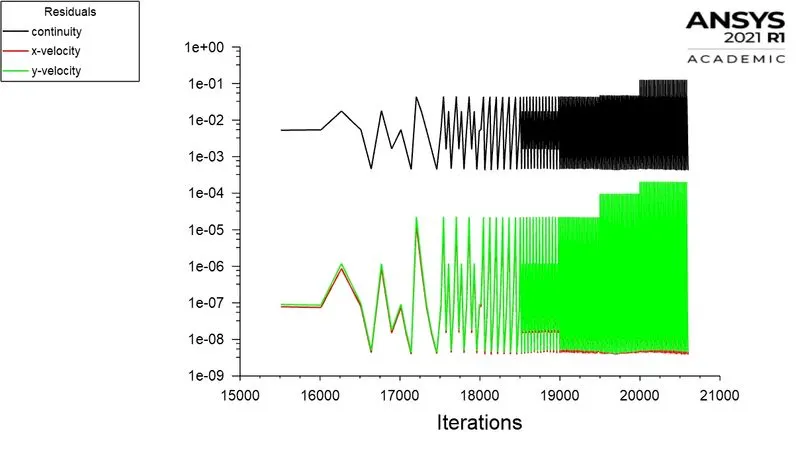
A transientstate solver with the laminar viscous model has been used to simulate the problem. The SIMPLE scheme with the least square cell-based system for gradients is used. Pressure and momentum interpolation schemes were chosen as second- order upwind. The B.C at inlet velocity is 1m/s. At outlet , pressure-outlet conditon is used with gauge pressure equals to zero. At the walls the no-slip condition is given and the bottom nd top boundaries were treated with symmetry B.C.
Reference values:
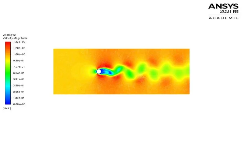
Velocity Contour:
Pressure Contour:
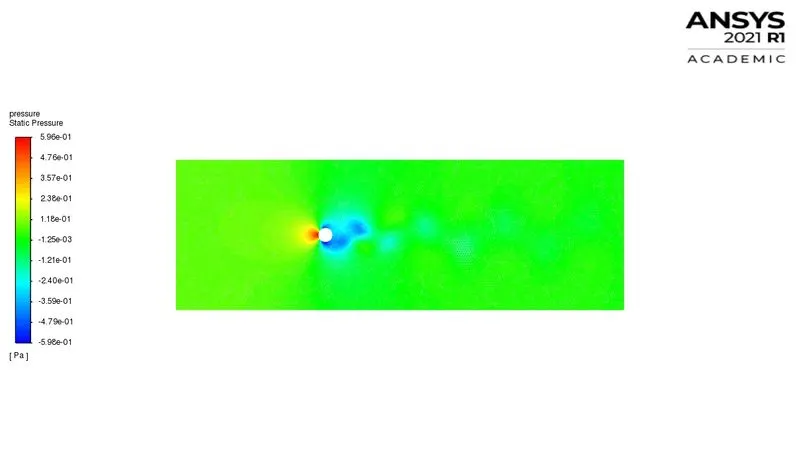
Residual plot:
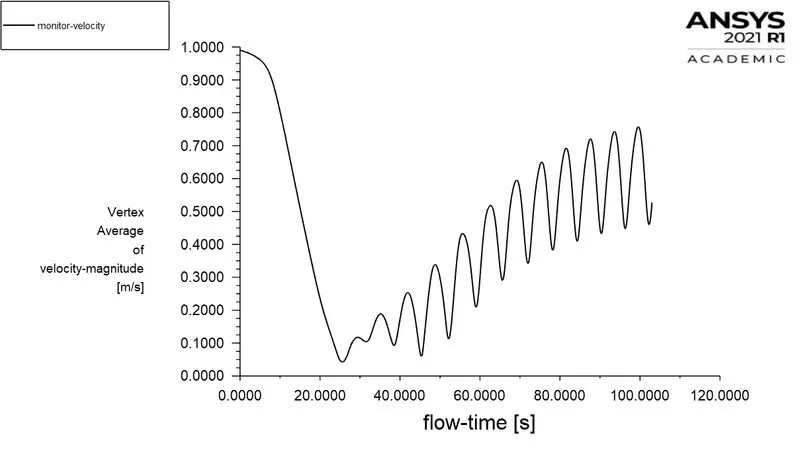
Vertex average velocity plot:
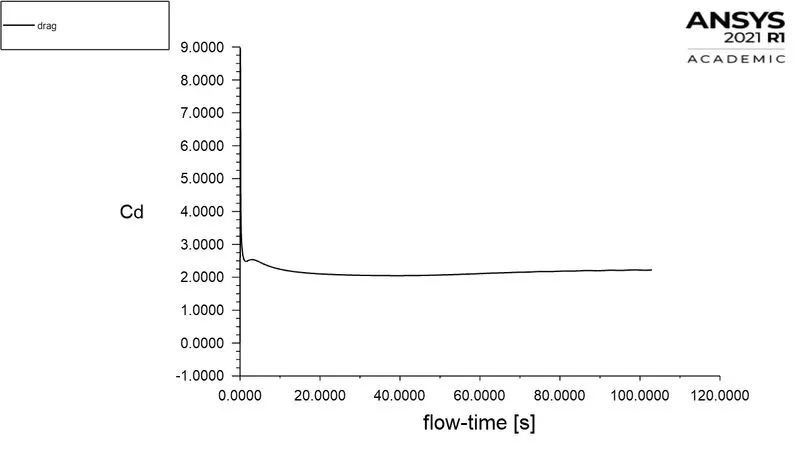
Coefficient of drag plot:
Coefficient of lift plot:
Strouhal number plot:
Solution animation:
| Solver | Cd | Cl | Strouhal number |
| Steady-state | 1.365 | -0.13 | 0.01333 |
| Unsteady-state | 1.336 | -1.179 | 0.1996 |
PART-2:-
Re=10
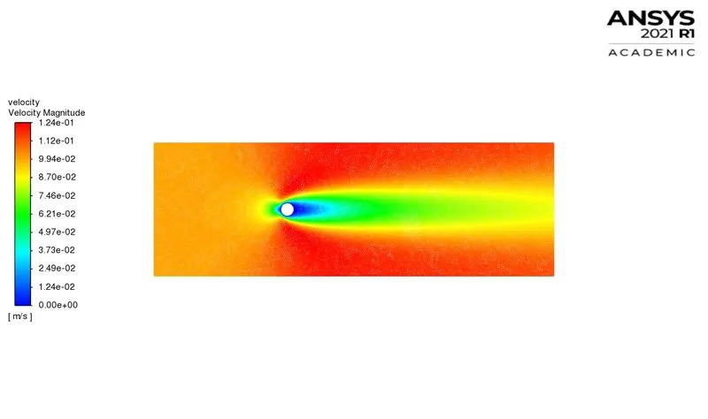
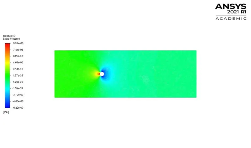
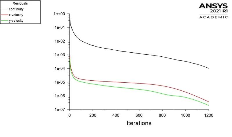
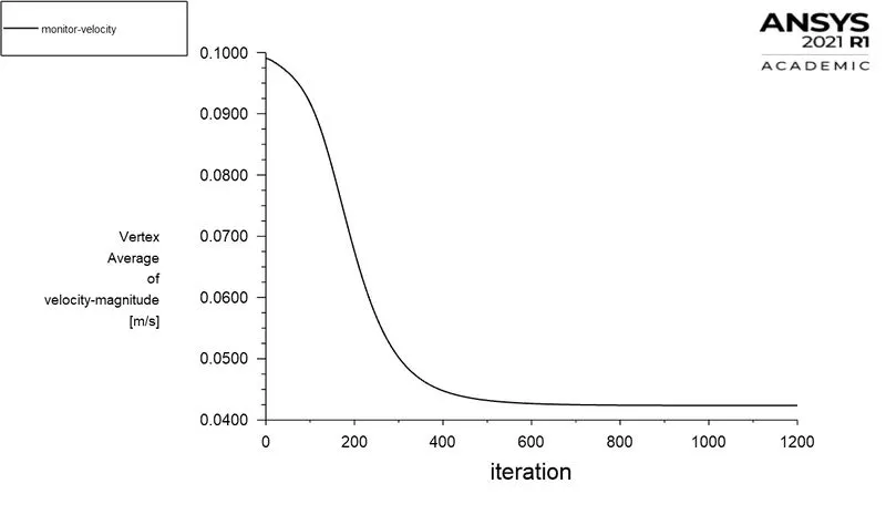
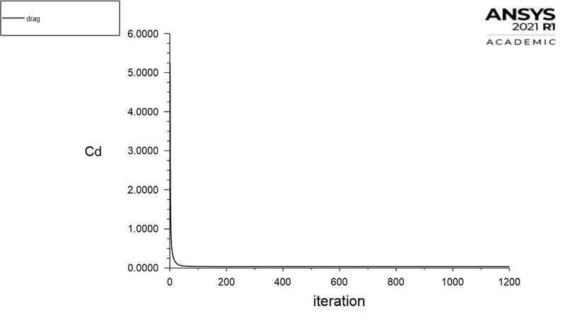
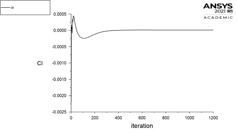
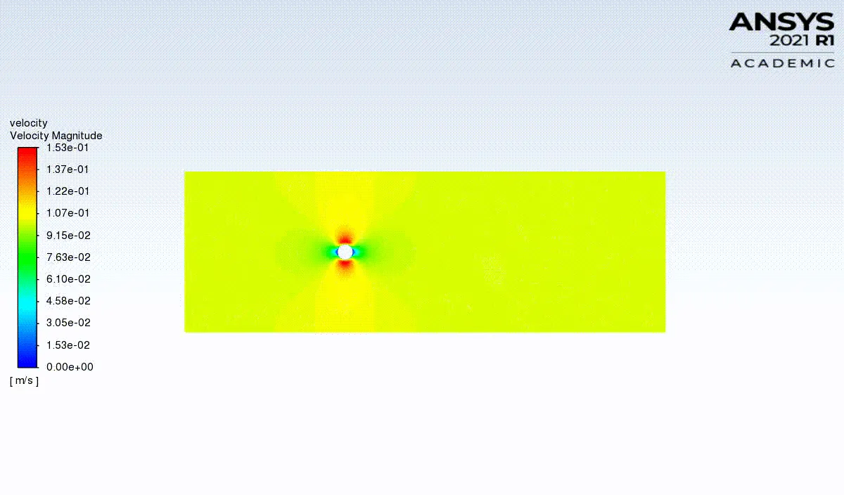
A steady state solver with the laminar viscous model has been used to simulate the problem. The SIMPLE scheme with the least square cell-based system for gradients is used. Pressure and momentum interpolation schemes were chosen as second- order upwind. The B.C at inlet velocity is 0.1m/s. At outlet , pressure-outlet conditon is used with gauge pressure equals to zero. At the walls the no-slip condition is given and the bottom nd top boundaries were treated with symmetry B.C
Reference values:
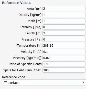
The results are given below.
Velocity Contour:
Pressure Contour:
Residual plot:
Vertex average velocity plot:
Coefficient of drag plot:
Coefficient of lift plot:
Solution animation:
Re=100
A steady state solver with the laminar viscous model has been used to simulate the problem. The SIMPLE scheme with the least square cell-based system for gradients is used. Pressure and momentum interpolation schemes were chosen as second- order upwind. The B.C at inlet velocity is 1m/s. At outlet , pressure-outlet conditon is used with gauge pressure equals to zero. At the walls the no-slip condition is given and the bottom nd top boundaries were treated with symmetry B.C
Reference values:
The results are given below.
Velocity Contour:
Pressure Contour:
Residual plot:
Vertex average velocity plot:
Coefficient of drag plot:
Coefficient of lift plot:
Solution animation:
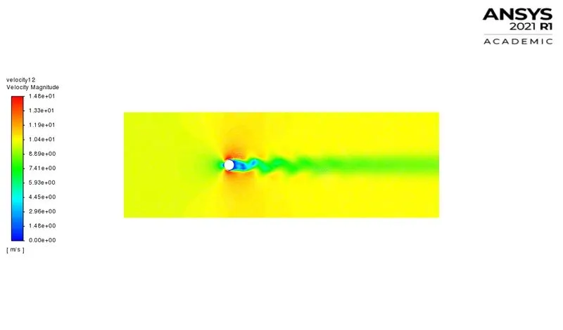
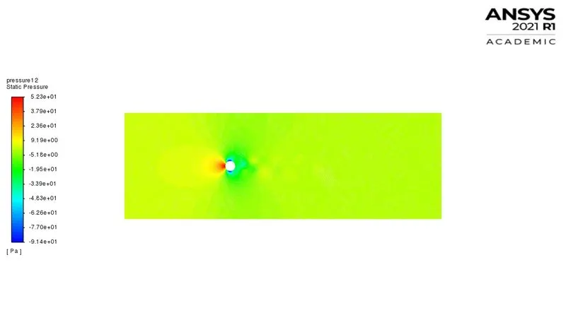
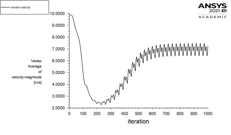
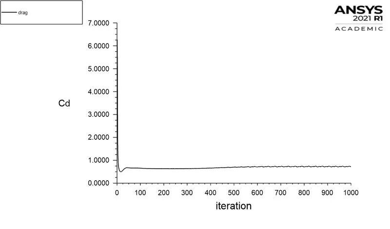
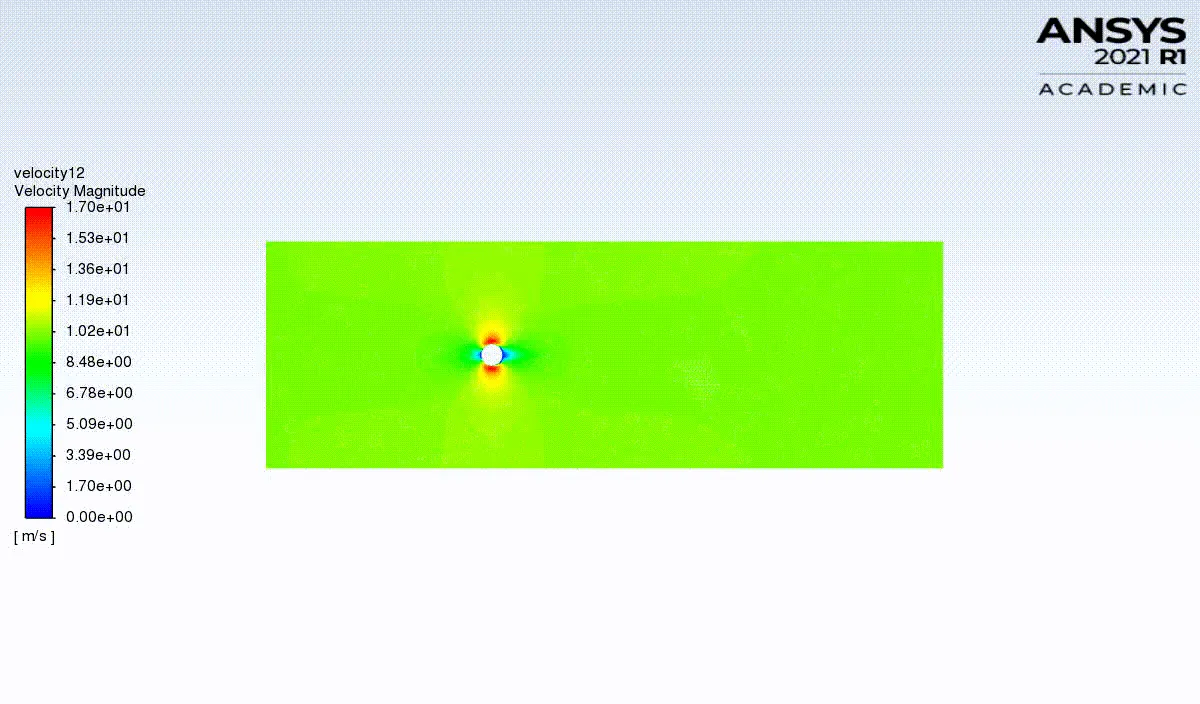
Re=1000
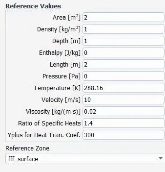
A steady state solver with the laminar viscous model has been used to simulate the problem. The SIMPLE scheme with the least square cell-based system for gradients is used. Pressure and momentum interpolation schemes were chosen as second- order upwind. The B.C at inlet velocity is 10m/s. At outlet , pressure-outlet conditon is used with gauge pressure equals to zero. At the walls the no-slip condition is given and the bottom nd top boundaries were treated with symmetry B.C
Reference values:
The results are given below.
Velocity Contour:
Pressure Contour:
Vertex average velocity plot:
Coefficient of drag plot:
Coefficient of lift plot:
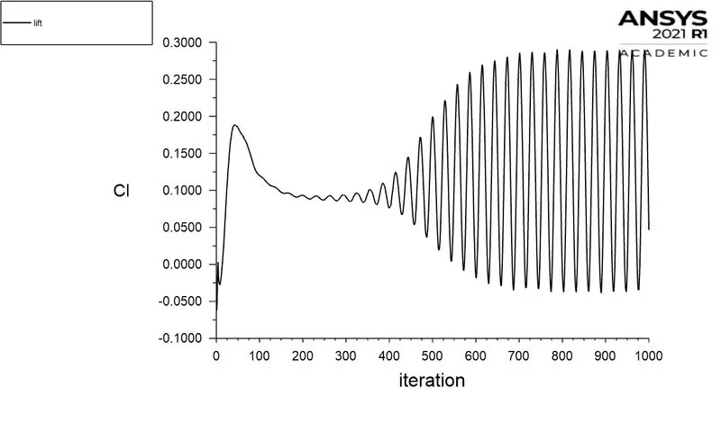
Solution animation:
Re=10000
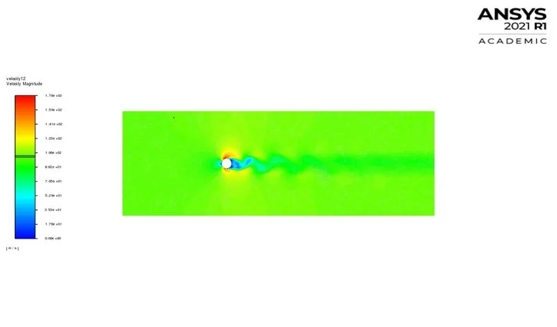
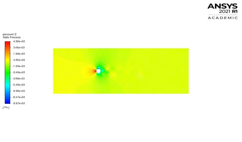
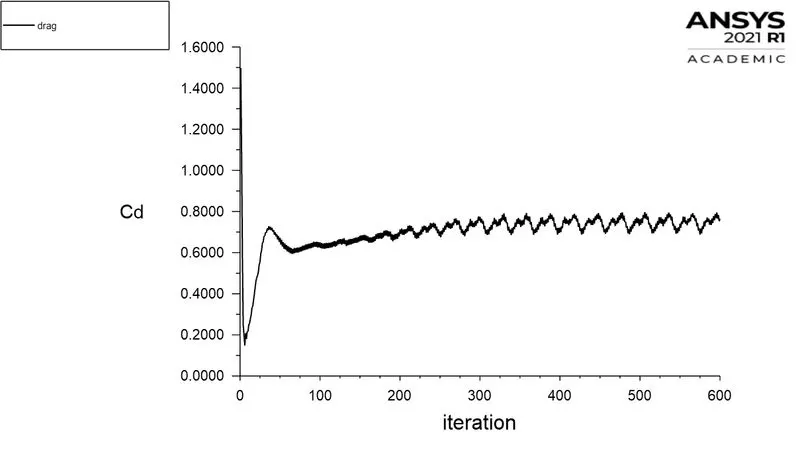
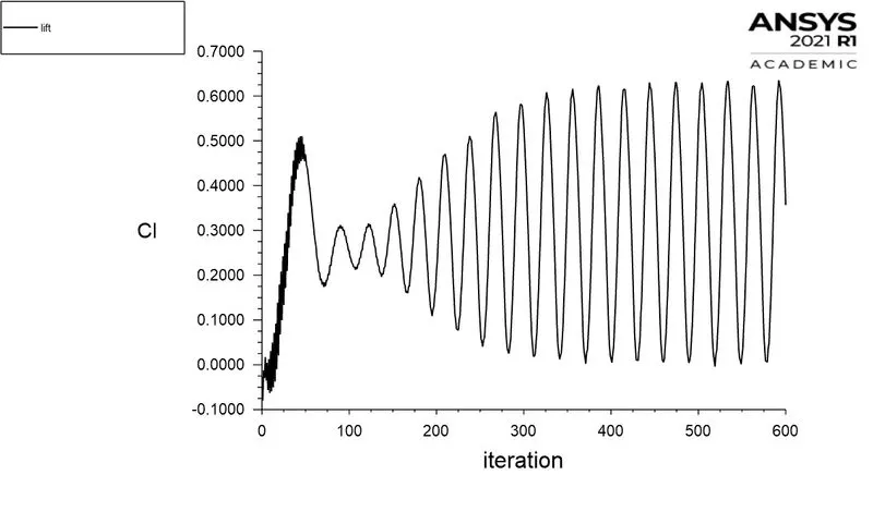
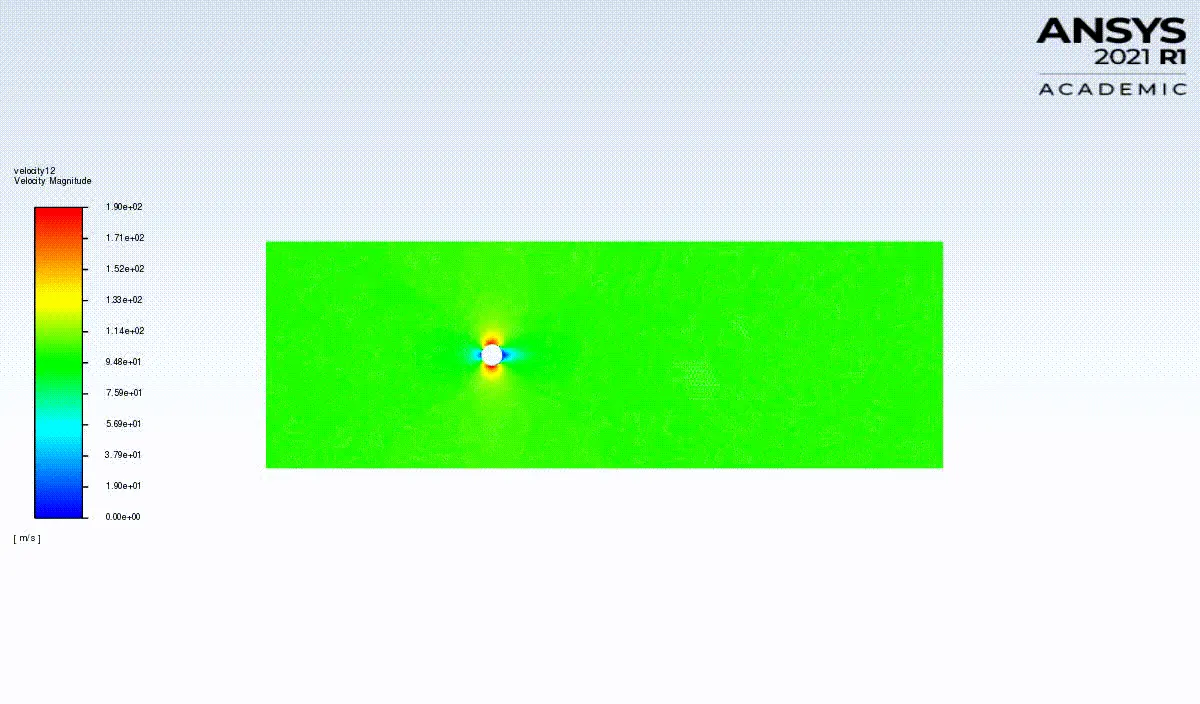
A steady state solver with the laminar viscous model has been used to simulate the problem. The SIMPLE scheme with the least square cell-based system for gradients is used. Pressure and momentum interpolation schemes were chosen as second- order upwind. The B.C at inlet velocity is 100m/s. At outlet , pressure-outlet conditon is used with gauge pressure equals to zero. At the walls the no-slip condition is given and the bottom nd top boundaries were treated with symmetry B.C
The results are given below.
Velocity Contour:
Pressure Contour:
Coefficient of drag plot:
Coefficient of lift plot:
Solution animation:
Re=100000
A steady state solver with the laminar viscous model has been used to simulate the problem. The SIMPLE scheme with the least square cell-based system for gradients is used. Pressure and momentum interpolation schemes were chosen as second- order upwind. The B.C at inlet velocity is 1m/s. At outlet , pressure-outlet conditon is used with gauge pressure equals to zero. At the walls the no-slip condition is given and the bottom nd top boundaries were treated with symmetry B.C
The results are given below.
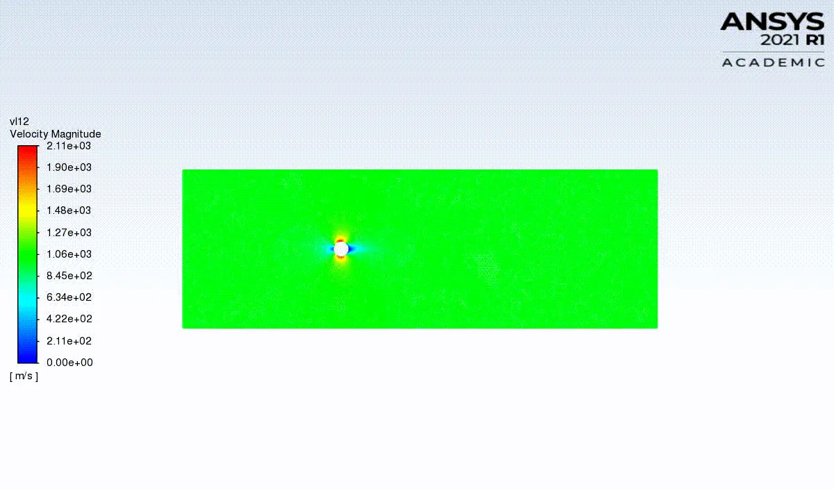
Velocity Contour:
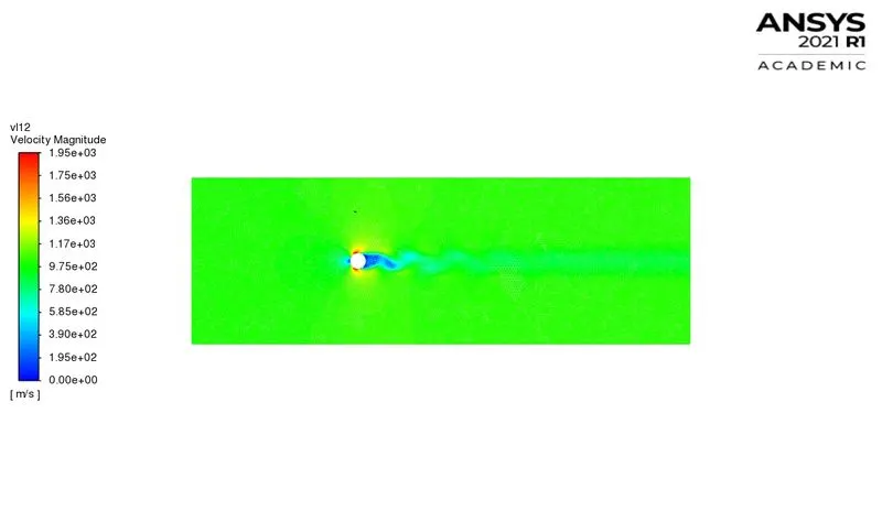
Pressure Contour:
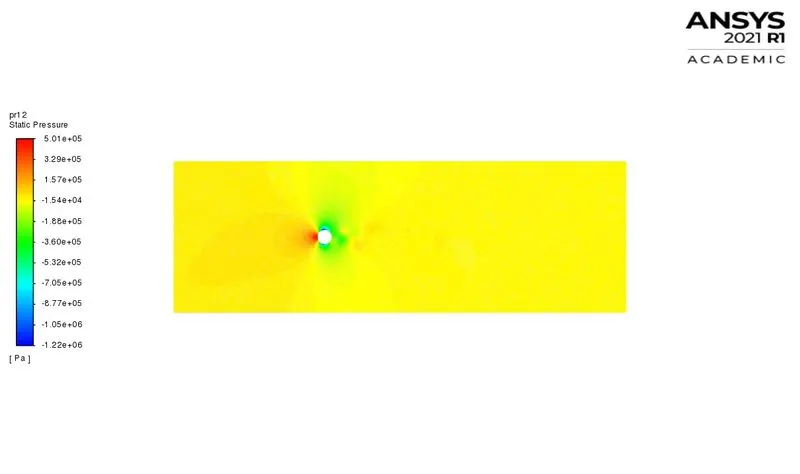
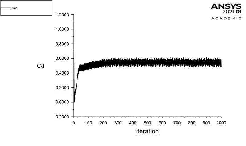
Coefficient of drag plot:
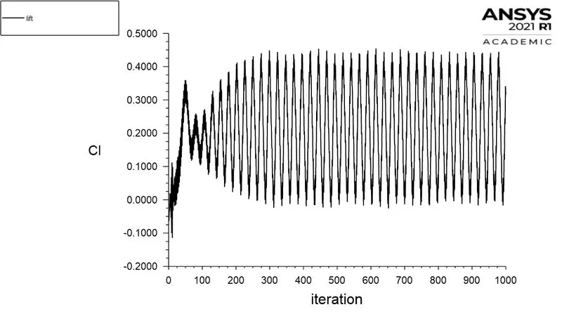
Coefficient of lift plot:
Solution animation:
| Reynolds number | Inlet velocity(m/s) | Co-efficient of drag | Co-efficient of lift |
| 10 | 0.1 | 1.0588 | 0.0002934 |
| 100 | 1 | 0.426 | 0.0056 |
| 1000 | 10 | 0.2371 | 0.04129 |
| 10000 | 100 | 0.2465 | 0.1081 |
| 100000 | 1000 | 0.1799 | 0.088114 |
Conclusion:
As the reynolds number is increased the vortices are shed alternately from the upper and lower surface of the cylinder at a definite frequency which is a function of reynolds number. When the reynolds number becomes greater than 1000 the oscillations were found to be increasing i.e, as the reynolds number becomes increases, interial forces dominate over the viscous forces. The co-efficient of drag (Cd) is found to be decreasing and the oscillatory nature of the co-efficient of lift is observed. The mean of vertex avergae of velocity and co-efficient of lift is found to be increasing with reynolds number.
From the table, we can notice that as we increase the Reynolds number our drag co-efficient is decreasing where as the lift co-efficient increasing. When we compre these results with the Rajani et al.[2], We found that our results agreed reasonably well.
But Contrastingly the drag co-efficient for Re=10000case should be less than of Re=1000 case and the values of the lift coefficient should be less than the values obtained from the Re=1000000 simulation.
It can be observed that along with an increase in the reynolds number, the flow becomes more and more unsymmetrical. Increasing velocity eventually brings the turbulent drag up to and even higher than the laminar drag value.
References:
https://en.wikipedia.org/wiki/K%C3%A1rm%C3%A1n_vortex_street
B.N Rajani, A. Kandaswamy, Sekhar Manjumdar