Week 10 - MRF project

Aim:

The given MRF model is unpacked and fluid blocks are created and analysis is performed for an accurate results when compared to an in-built fan model.

Objective:

The main objective of this project is to provide analysis and standards for the MRF fan modeling techniques for Moving Reference Frames(MRF) in ANSYS Icepak for the given CAD model.

Introduction for the Moving Reference Frame (MRF):

A Moving Reference Frame (MRF) is a relatively simple, robust, and efficient steady-state, Computational Fluid Dynamics (CFD) modeling technique to simulate rotating machinery. For example, the rotors on a quadcopter can be modeled with MRFs.

An MRF assumes that an assigned volume has a constant speed of rotation and the non-wall boundaries are surfaces of revolution (e.g., cylindrical, spherical, conical). In the case of the quadcopter example, the volumes between the rotor blades are designated as MRFs, assigned rotational speeds, and embedded within the multi-volume flow domain.

MRF is equivalent to running a rotational simulation and then observing the results at the instant equivalent to the position of the rotor within the MRF. MRF assumes a weak interaction between the MRF volume and the surrounding stationary volumes.

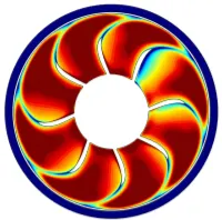
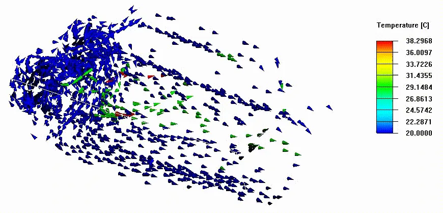
MRF CFD Simulation of Ducted Fan Shows velocity vectors within MRF volumes.

An alternative to MRF is the moving/sliding mesh technique, which can deal with strong interactions between the moving volume and the surrounding stationary volumes. However, in practice, the moving mesh technique often has robustness problems due to its dependence on intersection calculations between the stationary and rotating volumes. Also, the moving mesh technique is a transient (unsteady) simulation procedure which typically results in extremely long runtimes. Given the significant drawbacks of the moving mesh technique, the MRF is the preferred approach within its limitations.

Limitations for the MRF model:

Translation and rotational velocities are assumed to be constant (it is not allowed to vary in time.)

The specification of the relative velocity can not be used in conjunction with the MRF and mixture models. The absolute velocity definition is used instead for these situations. You don't need to have a single interface between reference frames where part of the interface consists of a two-sided coupled wall, while another part is not coupled. (i.e the normal interface treatment).

In such cases, the interface must be broken down into two interfaces: This is a coupled interface and the other is a fluid-fluid regular interface.

Flow chart:

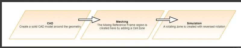
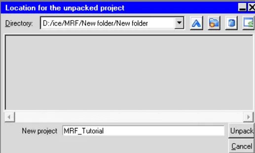
The model is unpacked with the given .tzr file

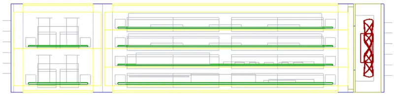
Below is the unpacked model geometry

Geometry:

now we have to create the fluid blocks around the fan blades

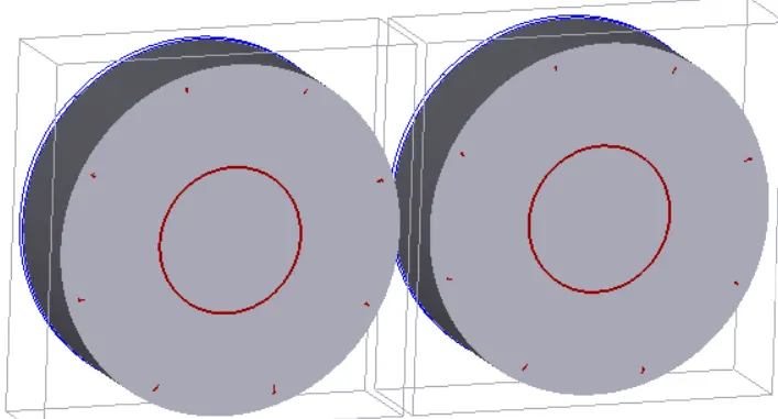
geometry of fluid blocks is shown below

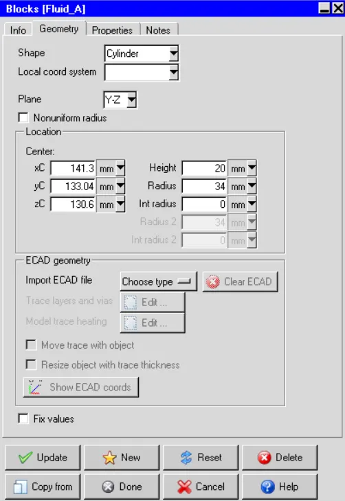
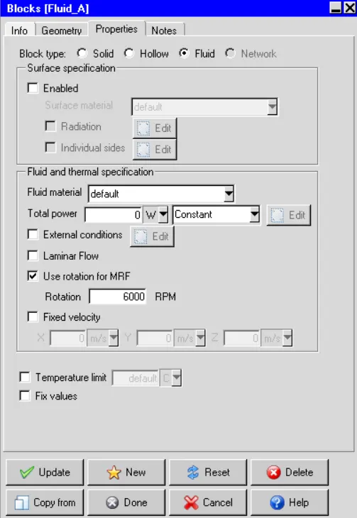
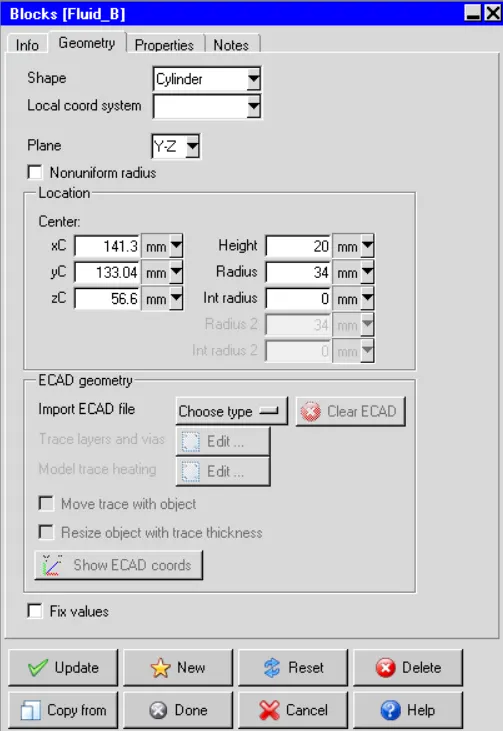
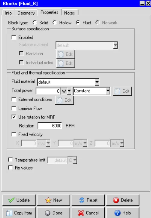
we can see the fan blades here

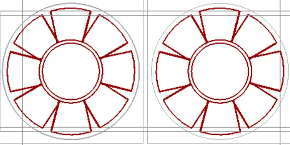
Fluid blocks covers both the fan blades A and B

Meshing:

An assembly is made such that Fluid blocks having higher priority than fan blades

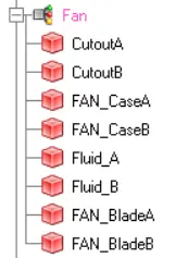
The following meshing techniques are utilized in the current project to discretize the computational domain:

Non-conformal meshing technique allows the user to selectively refine the mesh within a sub-region around an assembly by selecting the "Mesh separately" option available in the "Meshing" tab of the assembly settings. A comparatively normal mesh can be used for the rest of the model. Multiple assemblies, that employ non-conformal meshing, are defined in the model. The image attached below shows the settings applied in the "Meshing" tab to define one such assembly.

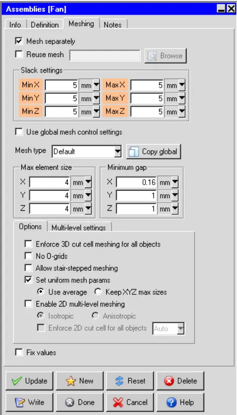
Multi-level mesh settings are enabled

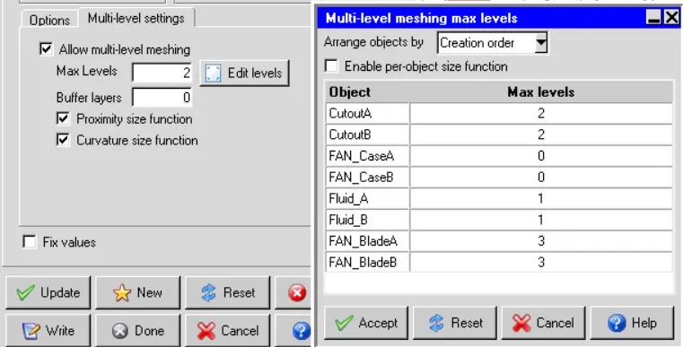
Further Assemblies can be created for racks of PCBs in order to reduce the mesh count

After completing the above steps, the computational mesh is generated. The image attached below shows the "Mesh control" window.

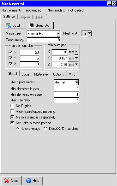
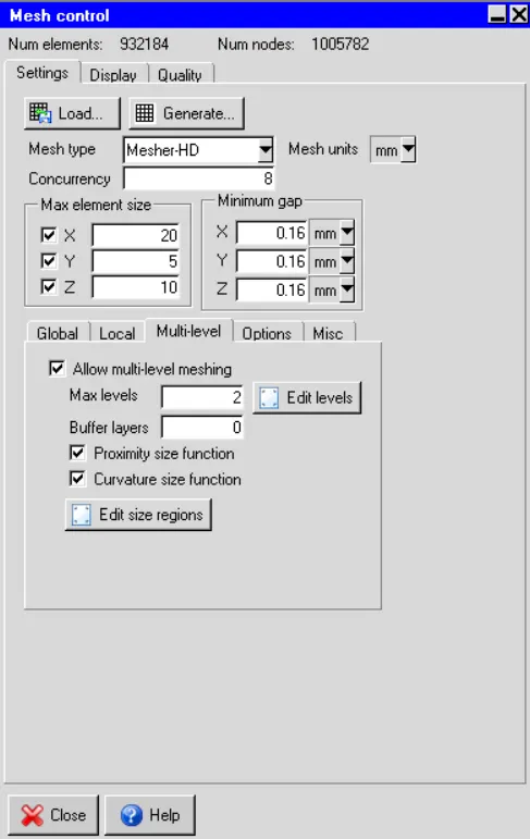
The image shows that the generated mesh yields 932184 elements and 1005782 nodes. The images attached below show the computational mesh on three mutually perpendicular planes, each passing through the center of the cabinet.

Z-plane

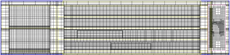
Y-plane

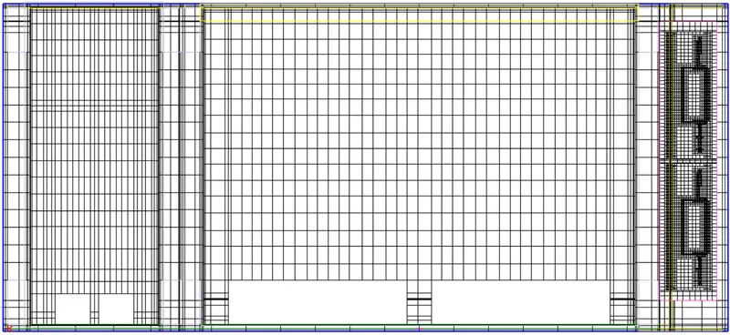
X-plane

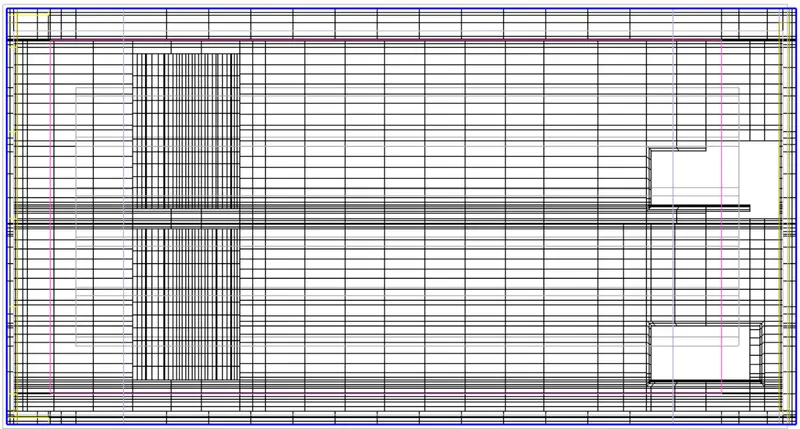
CAD model

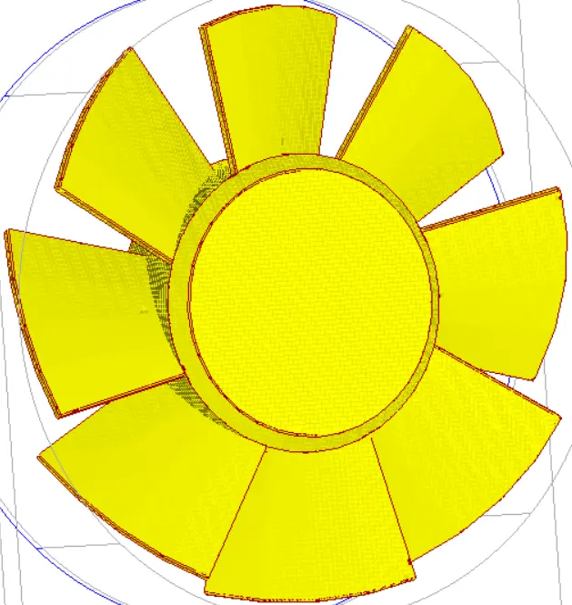
Visually the mesh appears to be fine. The images attached below show the histograms with the number of elements plotted.

Face-alignment

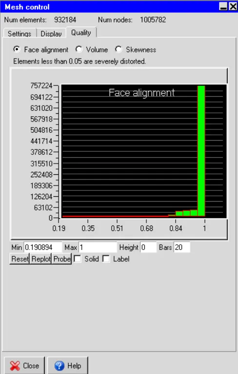
Values less than 0.05 indicate the presence of severely distorted elements in the mesh.

Volume

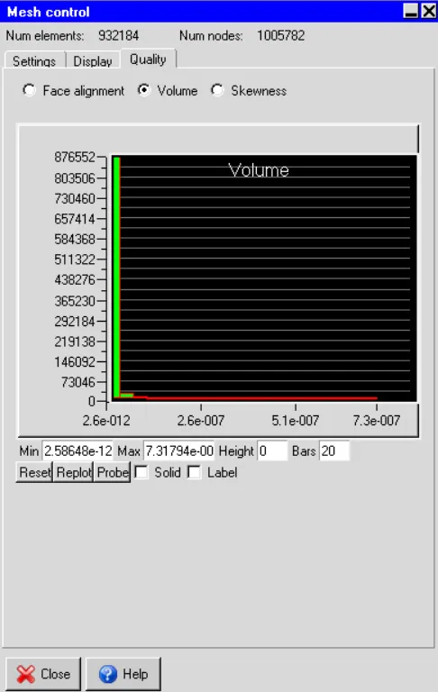
For a double precision solver, the minimum cell-volume shouldn't be less than 1e-15 m^3 otherwise the solver may face issues.

Skewness

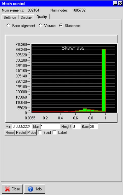
A skewness of 0 indicates that the mesh element is degenerate whereas a skewness of 1 indicates that the mesh element is ideal (equilateral/equiangular). All the elements in the current mesh have a skewness of 1 which indicates that they are ideal (equilateral/equiangular).

Solver:

The three-dimensional steady-state Navier-Stokes equations for the model are solved within the computational domain using the Fluent solver available in ANSYS Icepak. The following settings are applied to the solver:

1. Variables solved: Flow (velocity, pressure) and Temperature

2. Radiation: Off

3. Flow regime: Turbulent

3.1. Model: Realizable two equation model

4. Time variation: Steady

5. Solution initialization

5.1. X velocity: 0

5.2. Y velocity: 0

5.3. Z velocity: 0

5.4. Temperature: Ambient (20 deg. C)

6. Density model: Boussinesq approximation

6.1. Operating pressure: 101325 N/m2

7. Number of iterations: 1000

8. Convergence criteria

8.1. Flow: 1e-5

8.2. Energy: 1e-7

8.3. Joule heating: 1e-7

9. Configuration: Parallel

10. Number of processors: 4

11. GPU computing: Enabled

12. Number of GPUs: 1

13. Discretization scheme

13.1. Pressure: Standard

13.2. Momentum: First

13.3. Temperature: First

14. Under-relaxation factors

14.1. Pressure: 0.3

14.2. Momentum: 0.7

14.3. Temperature: 1

14.4. Viscosity: 1

14.5. Body forces: 1

14.6. Joule heating potential: 1

15. Linear solver settings

15.1. Pressure - Type: V, Termination criterion: 0.1, Residual reduction tolerance: 0.7, Stabilization: None

15.2. Momentum - Type: flex, Termination criterion: 0.1, Residual reduction tolerance: 0.7

15.3. Temperature - Type: F, Termination criterion: 0.1, Residual reduction tolerance: 0.7, Stabilization: None

15.4. Joule heating potential - Type: W, Termination criterion: 1e-6, Residual reduction tolerance: 0.7, Stabilization: None

16. Precision: Double

Results:

In the current section, the simulation results are discussed.

Residuals:

The residuals of the following equations are plotted against the number of iterations:

i. Continuity equation

ii. X-Momentum equation

iii. Y-Momentum equation

iv. Z-Momentum equation

v. Energy equation

The image attached below shows the residuals plotted against the number of iterations.

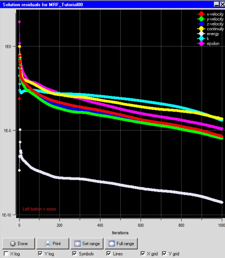
The plot shows that the residuals are quite small quantitatively and don't change appreciably between 800-1000 iterations thereby indicating that the solution has reached a steady state. In the current project, the simulation results after 1000 iterations are considered as steady-state results.

Monitor plots:

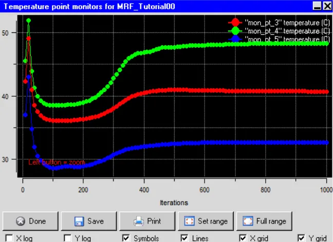
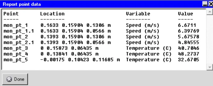
Monitor points are probes set up at various key locations within the computational domain to determine the solution variables (such as pressure, velocity, temperature etc.). Data obtained from monitor points can also be used to ascertain whether the solution has reached a steady state. In the current project the following monitor ponts are created

The images attached below show the data obtained from the monitor points, plotted against the number of iterations.

1.Temperature monitor points

i. mon_pt_3: Temperature monitor point

ii. mon_pt_4: Temperature monitor point

iii. mon_pt_5: Temperature monitor point

2.Velocity monitor points

i. mon_pt_1: Velocity monitor point @ Fan_blade_A

ii. mon_pt_1.1: Velocity monitor point @ Fan_blade_B

iii. mon_pt_2: Velocity monitor point @ Cutout_A

iv. mon_pt_2.1: Velocity monitor point @ Cutout_B

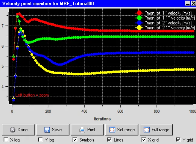
The plots show that the monitored values don't change appreciably after 500 iterations. This further confirms that the simulation results after 1000 iterations are steady-state results. The following steady-state values are predicted by the plots:

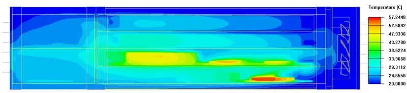
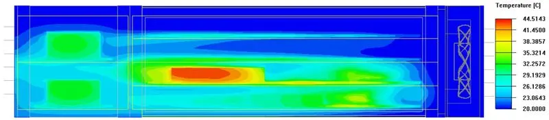
Temperature contours

The steady-state temperature contours are plotted on the Z-plane passing through the Fan blade A, as shown in the image attached below.

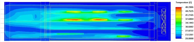
The steady-state temperature contours are plotted on the Z-plane passing through the Fan blade B, as shown in the image attached below.

The steady-state temperature contours are plotted on the Z-plane passing through the center of the cabinet, as shown in the image attached below.

Velocity vectors

The steady-state velocity vectors are plotted on the Z-plane passing through the center of the cabinet, as shown in the image attached below.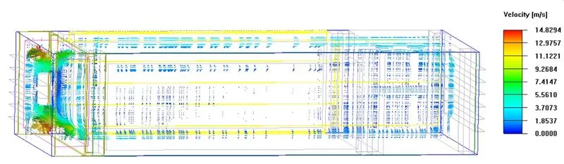

The plot shows the velocity vectors for air plotted at 1000 points distributed uniformly throughout the X-plane passing through the center of the cabinet.

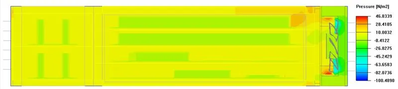
Pressure vectors

The steady-state velocity vectors are plotted on the Z-plane passing through the fan blade A, as shown in the image attached below.

The steady-state velocity vectors are plotted on the Z-plane passing through the centre of the cabinet, as shown in the image attached below.

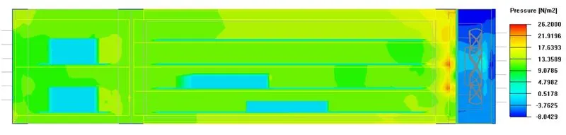
The steady-state velocity vectors are plotted on the Z-plane passing through the fan blade B, as shown in the image attached below.

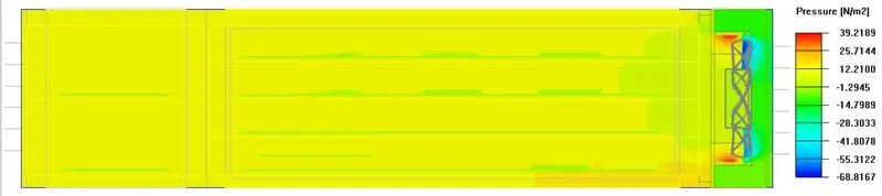
Velocity contours

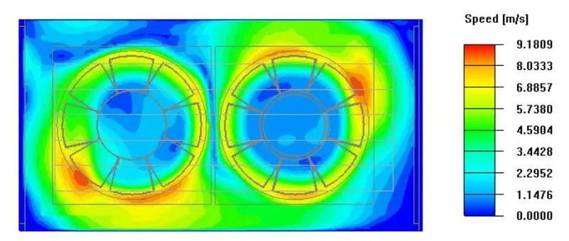
The steady-state velocity contours are plotted on the Z-plane passing through the fan blade A, as shown in the image attached below.

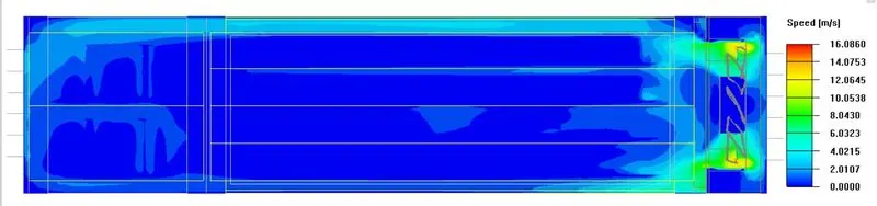
The steady-state velocity contours are plotted on the Z-plane passing through the center of the cabinet, as shown in the image attached below.

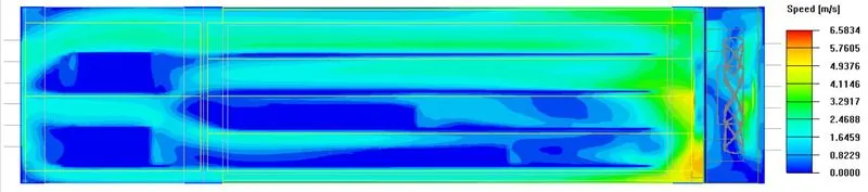
The steady-state velocity contours are plotted on the Z-plane passing through the fan blade B, as shown in the image attached below.

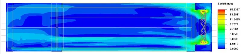
Here the velocity is specified between 0 to 3m/s

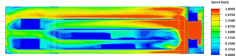
The steady-state velocity contours are plotted on the X-plane passing through the fan blades A & B, as shown in the image attached below.

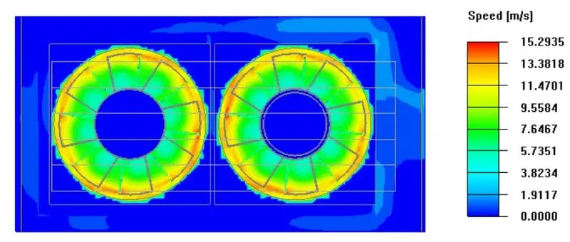
The steady-state velocity contours are plotted on the X-plane

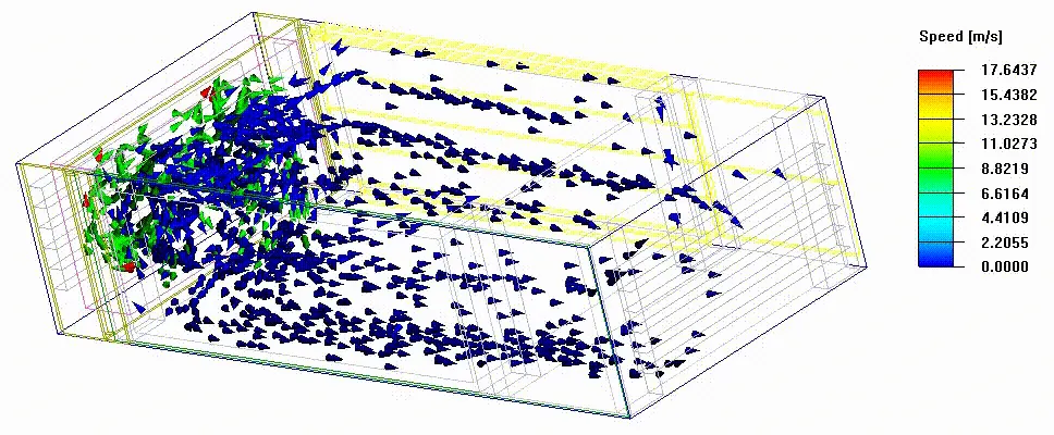
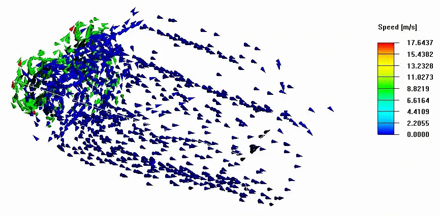
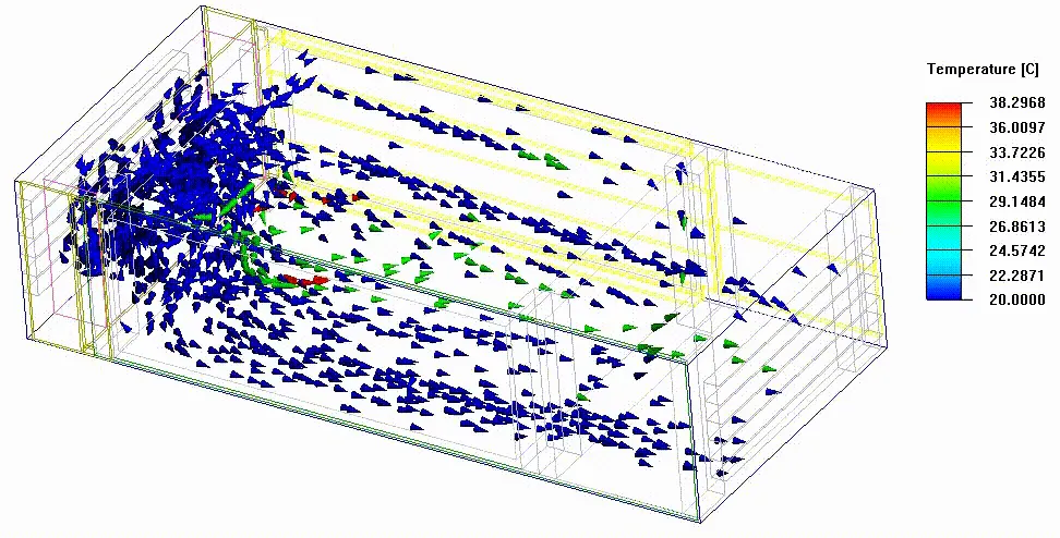
Particle traces:

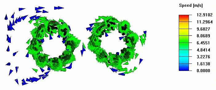
The steady-state particle traces (colored by temperature) of 500 particles

Here object face for grille2 is selected as flow is getting into the cabinet

Velocity

Temperature

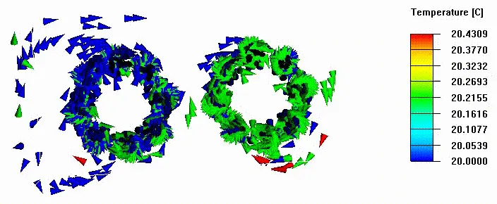
Velocity particles inside the cabinet

Without cabinet

Temperature particles inside the cabinet

without cabinet

Conclusion:

• Moving Reference Frame (MRF) modeling enables more accurate predictions of the flow.
• MRF reduces errors in predicting component temperatures because it directly throws the flow on to the components. This phenomenon we can't get through the normal modeling of the fan.
• MRF modeling is very accurate in predicting the flow, turbulence, and system noise levels.
• This model also gives accurate results of flow, temperature, and some other parameters even in high-density electronic models.