Week 4.1: Project - Steady state simulation of flow over a throttle body

Aim:

To simulate the flow over the throttle inside the elbow and to study pressure, velocity contours and plots for pressure, velocity, mass flow rate and total cell count.

Throttle:

A throttle is the mechanism by which fluid flow is managed by constriction or obstruction. An engine's power can be increased or decreased by the restriction of inlet gases by the use of a throttle. The throttle refers to any mechanism by which the power or speed of an engine is regulated, such as a car's accelerator pedal. In the current simulation the throttle is kept constant at the initial position and the steady state simulation is carried out to study the variation of fluid flow quantities due to throttle.

Case Setup:-

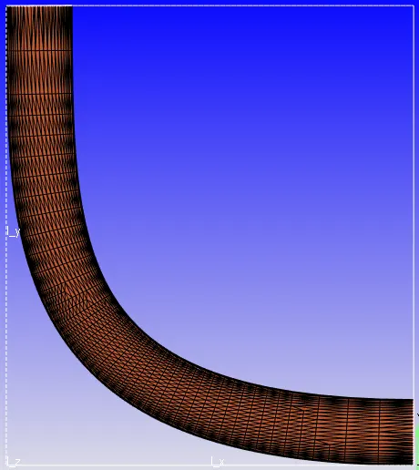
1. Geometry Creation:- The geometry that was used for the analysis is shown below. An STL file was imported into CONVERGE. It comprised of a number of open edges that were cleaned using a Patch command.

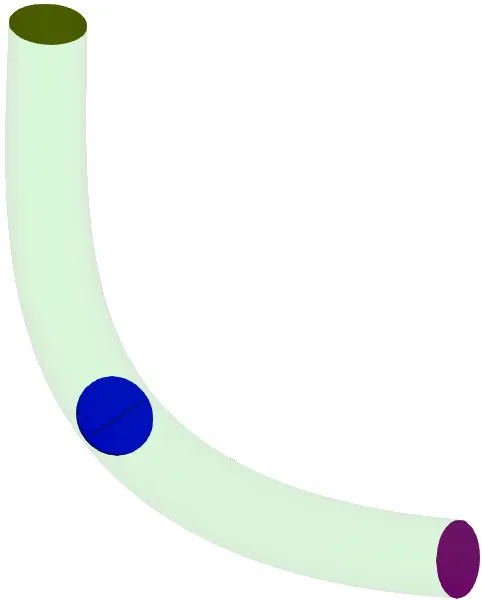
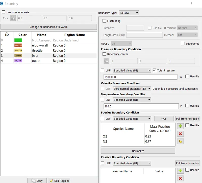
1. Creation of Boundaries: In the geometry which is created above, boundaries such as inlet, outlet , outer body and throttle.

1. Checking Orientation of Normals:Orientation of Normals were checked to ensure all the normals are pointing inwards. This was done using the Normal Toggle
2. Finally a Diagnosis check was run to ensure no errors in the geometry.

Case Setup:

• Application Type:- This was set to Time based
• Materials: This was set to Air

Gas Simulation: Default properties were retained

Global Transposrt Parameters:- Default properties retained

1. Species : Add N2 and O2 in Gas.

• Simulation Parameters:

  Run parameters:

  Solver : Steady- State solver

  Simulation mode: Full hydrodynamic

  Turn off use shared memory and turn on steady state monitor Misc tab.

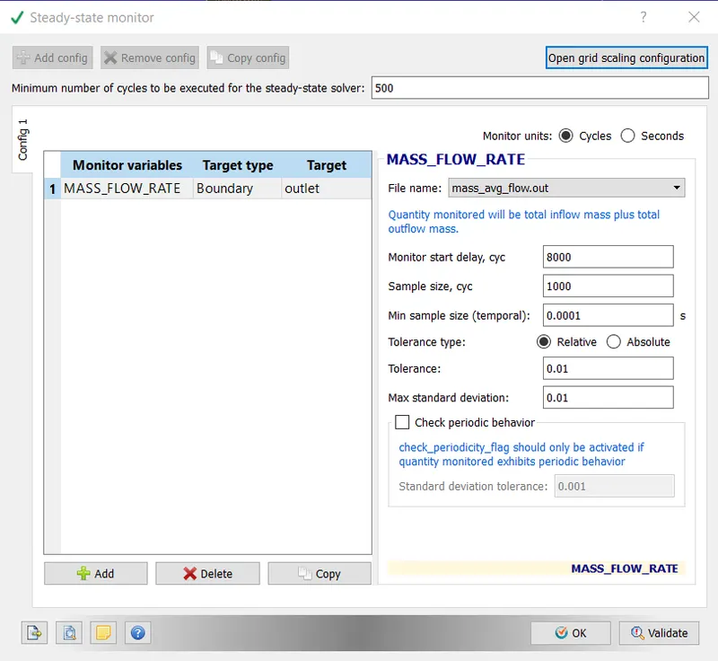
  Steady State Monitor:

  Add required parametres that need to be monitored so that if they converge within the given tolerance value the simulation would stop before reaching the given number of cycles to complete(End time)

• Boundary Conditions:

Inlet

Boundary type - INFLOW.

Pressure - 150000 Pa

Temperature - 300 K

Species - N2 = 0.77 and O2 = 0.23

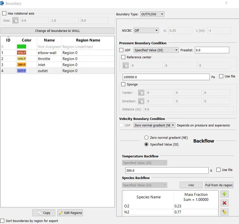
Outlet

Boundary type - OUTFLOW.

Pressure - 100000 Pa

Temperature - 300 K

Species - N2 = 0.77 and O2 = 0.23

This pressure difference between inlet and Outlet drives the flow from inlet and outlet .Also mention O2 and N2 species dor Backflow ( if it occurs due to adverse pressure)

• Throttle

Since throttle is not moved/rotated in this case

Boundary type - WALL

Wall motion : Stationary

Apply Law of Wall for Velocity and Temperature Boundary Conditions.

• Elbow_Wall

Boundary type - WALL

Wall motion : Stationary

Apply Law of Wall for Velocity and Temperature Boundary Conditions.

• Simulation Time Parameters:

  Start time - 0

  End time - 15000 cycles

  Intial time step : 1e-9 s

  Minimum time step:1e-9 s

  Maximum Time step: 1 s

  Maximum convection CFL limit: 1

  Leave the rest as Default values.

• Solver Parameters:

NS solver Scheme - PISO

NS Solver Type - Pressure Based Steady

Set the pre conditioner to none in Pressure in the Equation tab.

Set the maximum convection CFL limit to 0.5 in Steady state Solver Control tab and rest are left Default.

• Initial condition and events

The created geometry was selected as the Volumetric Region

• Physical Models:

Turbulence model : RNG k -ε">ε in RANS

• Grid Control :

Base grid : dx=dy=dx = 0.002 m

Add fixed Embedding in Grid control

Fixed Embedding was also enabled. This was done to capture the flow around the throttle valve with greater precision.

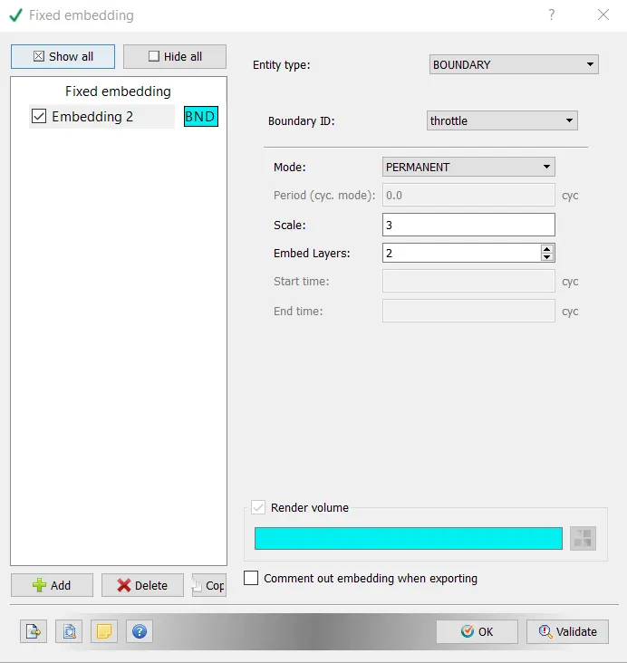
At the throttle major changes in the flow variables occur.. In Order to capture the results accurately at the throttle, fine mesh will be need with more cells. So mesh size is reduces at the throttle with tthe help of fixed embedding. Scale of 3 makes the reduces the base mesh size by 8(2^3) times and embedded lalayers 2 means the mesh size is further reduced by 8 times at the throttle boundary.

Output/Post-processing

In post variable selection, under SPecies tab, add N2 and O2 in mass fraction box.

In output files, under Writing time intervals tab, specify 100 cycles as time interval for writing 3D output data files and restarting files.

Export All these input files to a directory. Open CYGWIN, navigate to the directory where all these folders are saved and run the following command ;

mpiexec.exe -n 4 converge.exe restricted </dev/null> logfile_006 &

which runs the simulation with 4 processors using converge executable and outputs are dumped into a file called logfile_006 with job being ran in backend.

Outputs/Post -Processing:

Post processing is performed in the paraview software using the group files with ..vtm extension created in the post processor of Converge

Geometry:

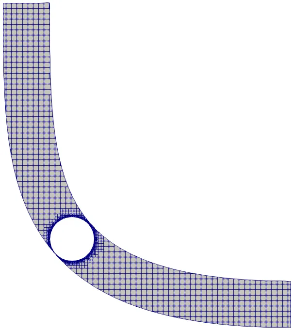
Finer Mesh at the Throttle

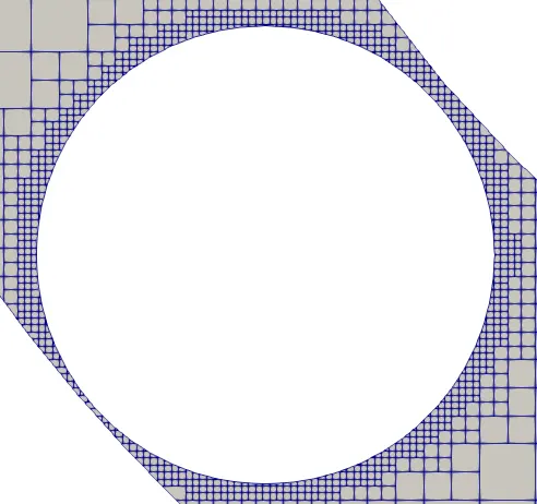
The finer mesh near throttle using the fixed embedding in order to obtain better results. The mesh on tge complete geometry can be seen.

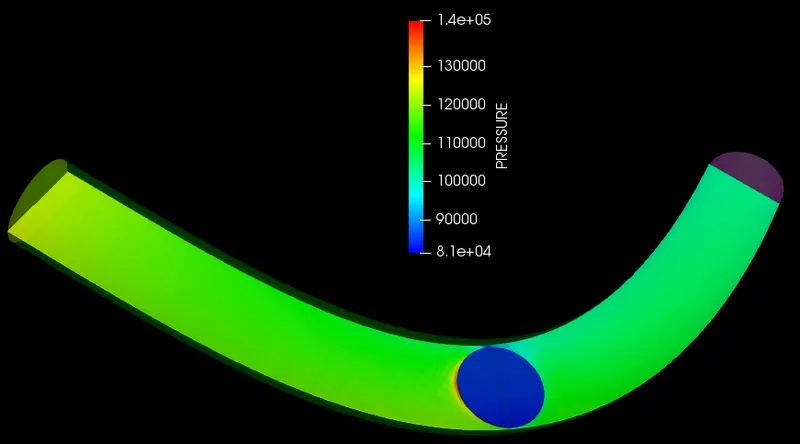
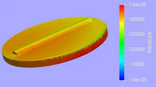
Pressure Contour:

Velocity contours

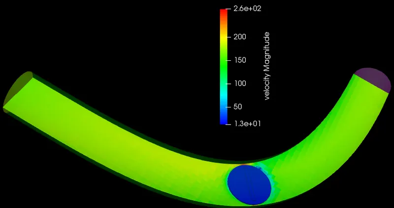
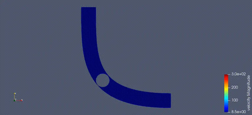
Steady-state velocity contours are plotted over a cut-plane.

Velocity vectors

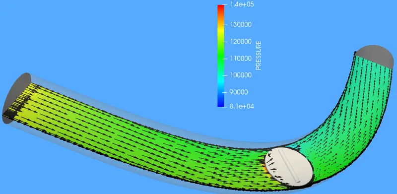
Steady-state velocity vectors are plotted over a cut-plane.

Animation:

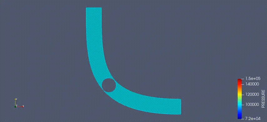
Pressure

Velocity

Outputs from the Plotting module of Converge:

Variation of flow quantities at Inlet and Outlet of geometry:

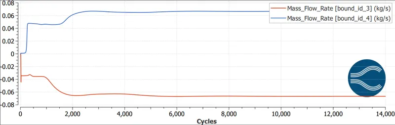
Mass Flow Rate:

Total Pressure:

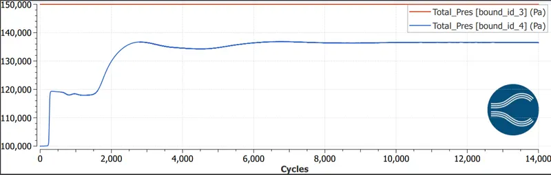
Increase in the total pressure at the outlet is due to the increased velocity of flow after the throttle which increases the dynamic pressure thereby total pressure. Velocity at inlet is the given initial condition of 150000 Pa.

Average Velocity:

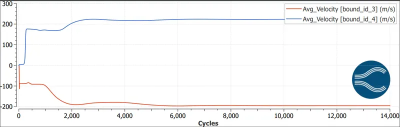
Average velocity at inlet is around 190m/s and 220 m/s at outlet

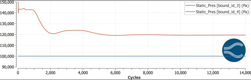
Static pressure:

Static pressure at inlet and outlet are plotted over simulation cycles.

Total Number of Cells:

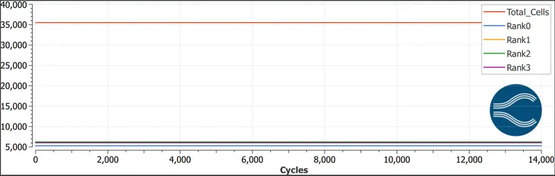
The simulation converges at around 6450 cycles and the number of cells is around 35500 inclusive of the given fixed embedding which resulted in more number of cells.

Conclusion:

1. The plot for mass flow rate indicates a good mass balance between inlet and outlet.

2. The plot for average velocity indicates that the average velocity at the outlet is 224.082m/s.

3. Pressure contours show maximum and minimum pressure values near the upstream and downstream locations of the throttle valve respectively.

4. Velocity contours show that a maximum velocity of 310m/s is achieved in the passage between throttle valve and pipe.