Week 5.3 - Forced convection Analysis

Aim:

To create workflow in ansys workbench and use the simplified geometry of DME assembly provided and solve them for physics using ansys icepak.

Introduction:

ANSYS Workbench platform is the backbone for delivering a comprehensive and integrated simulation. It is used to perform various types of structural, thermal, fluid, and electromagnetic analyses. The entire simulation process is tied together by a project schematic, from which you can interact with applications that are native to ANSYS Workbench or launch applications that are data-integrated with ANSYS Workbench. It includes CAD connectivity, automated meshing, a project-level update mechanism, optimization tools, DOE.

ANSYS Workbench is a project-management tool. It can be considered as the top-level interface linking all our software tools. Workbench handles the passing of data between ANSYS Geometry / Mesh / Solver / Postprocessing tools. This greatly helps project management. You do not need to worry about the individual files on disk (geometry, mesh, etc). Graphically, you can see at-a-glance how a project has been built.

It is easy to see at a glance how a model has been built, and determine which files were used for a particular simulation (pairing geometry files to solver runs). Workbench also makes it straightforward to perform parametric analyses (without the user needing to manually launch each application in turn), and makes it easy to simulate multi-physics scenarios like fluid-structure interaction.

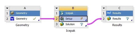
• Ansys Workbench uses the two types of CAD models, one is a design modeler and the other is SpaceClaim.
• Engineers in nowadays are mostly using the SpaceClaim because of the flexibility, compatibility, and having better and more handling options for the geometry.
• While a geometry or CAD file coming from a design section to the analysis section, it needs a lot of repair and modifications.

Geometry simplification:

The images attached below show the given CAD model of an electronic enclosure assembly.

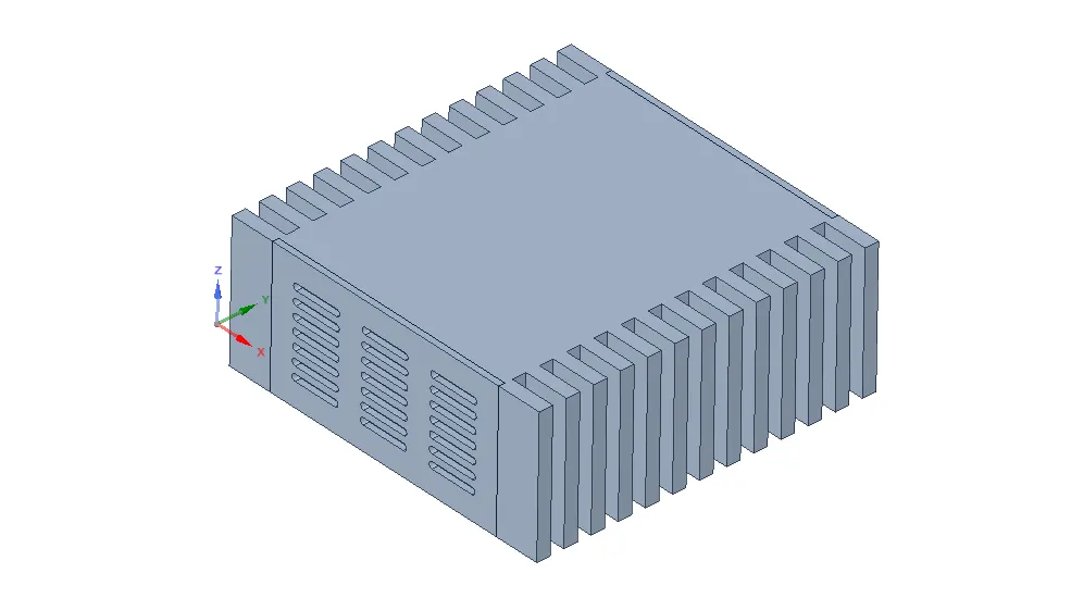
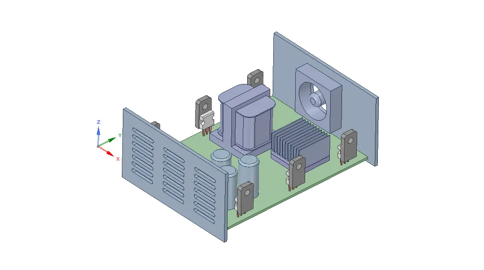
The following steps are used to simplify the given CAD model into an Icepak model

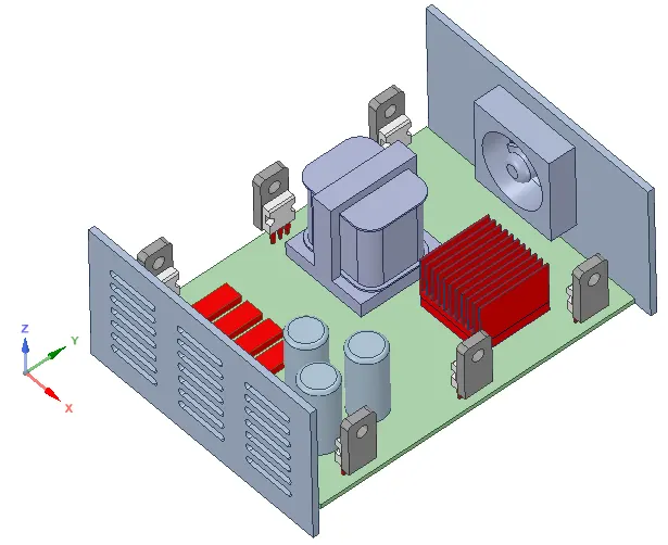
• "Identify Objects" command is used to simplify various objects in the model. The image attached below shows (in red color) the objects identified for simplification.

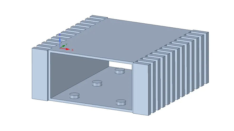
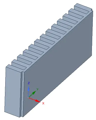
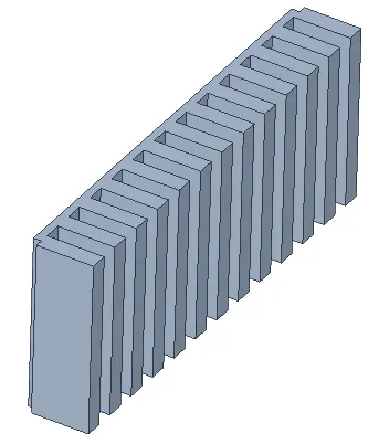
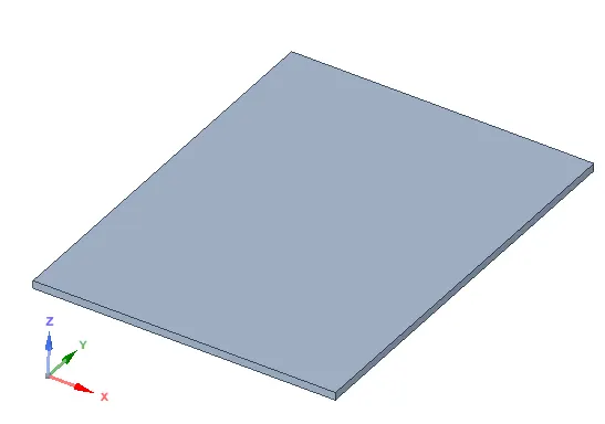
The housing is split intofour parts using two YZ planes. The images attached below show the housing before and after splitting.

Before splitting

After splitting

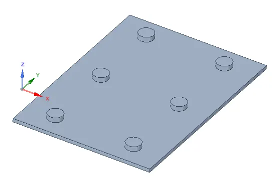
• The base of the housing is split further in order to separate the PCB supports from the housing.
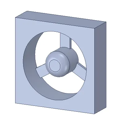
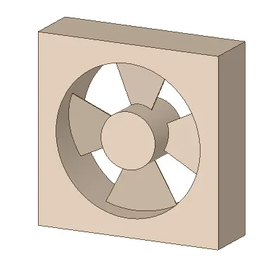
• The fan in the model is simplified using the "Fan" command. The images attached below show the fan before and after simplification.

Before simplification: After simplification

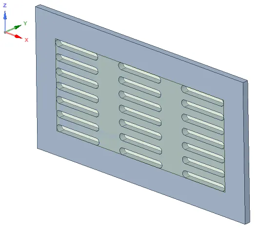
"Opening" and "Grille" commands are used to define an Icepak grille as shownin the image attached below.

The remaining objects in the model are simplified using "Icepak Simplify" command with different simplification types, namely: Level 0 (bounding box), Level 1 (cuboid, cylinder fit), Level 2 (polygon fit) and Level 3 (CAD object). The images attached below show the remaining objects in the model before and after simplification.

Coil:

Before simplification After Level 3 (CAD object) simplification

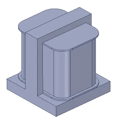
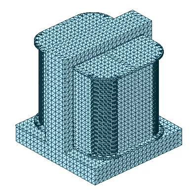
Finned part of the housing:

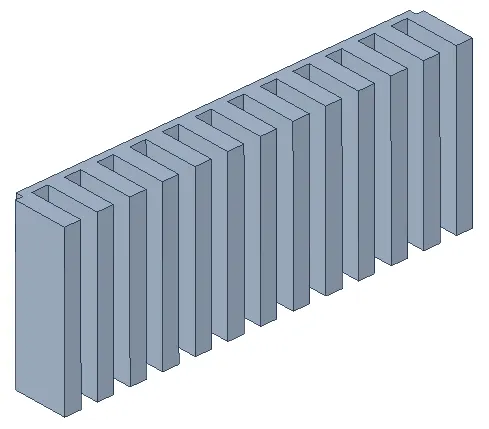
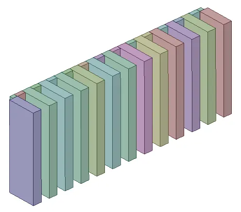
Before simplification After Level 1 (cuboid, cylinder fit) simplification

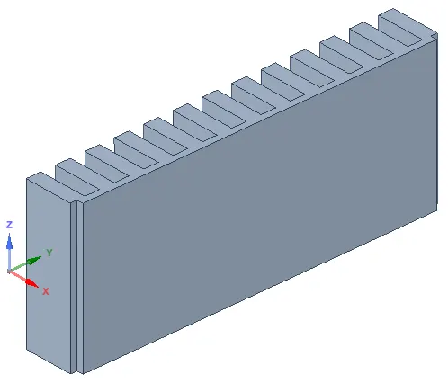
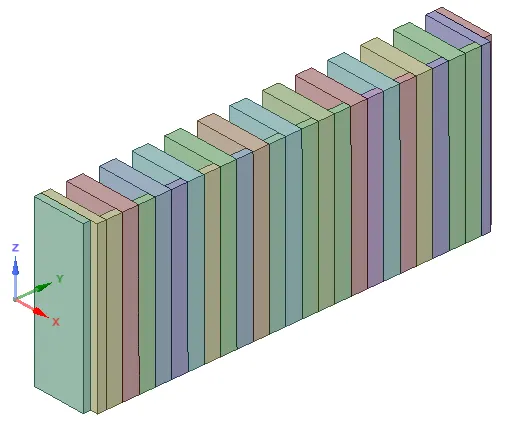
Finned part of the housing:

Before simplification After Level 1 (cuboid, cylinder fit) simplification

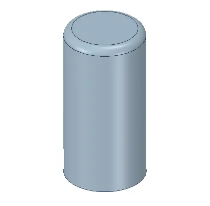
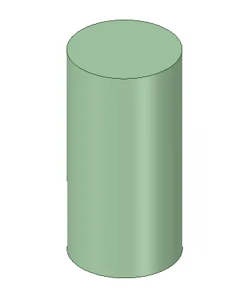
Capacitor:

Before simplification After Level 1 (cuboid, cylinder fit) simplification

Die casing:

Before simplification After Level 0 (bounding box) simplification

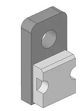
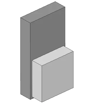
PCB:

Before simplification After Level 0 (bounding box) simplification

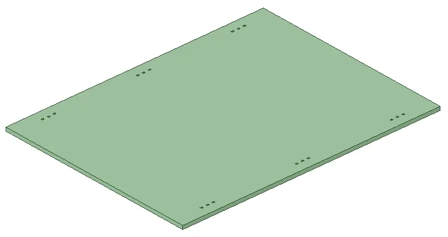
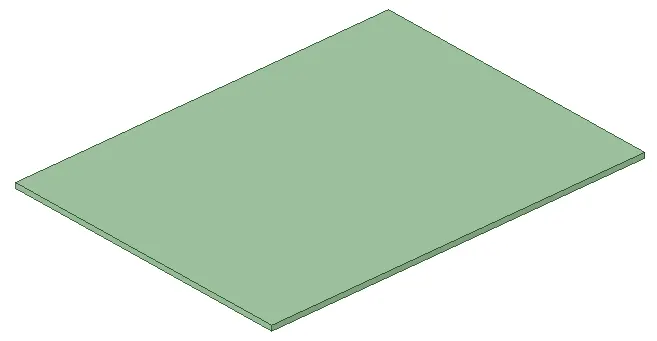
Top cover of the housing:

Before simplification After Level 0 (bounding box) simplification

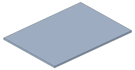
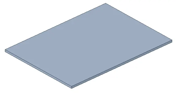
Bottom cover of the housing:

Before simplification After Level 0 (bounding box) simplification

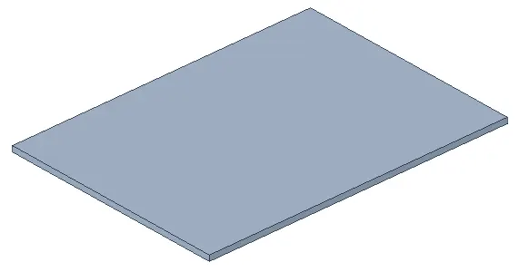
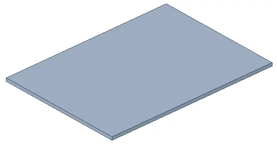
Rear-Panel of the housing:

Before simplification After Level 0 (bounding box) simplification

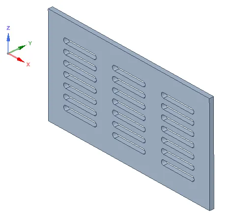
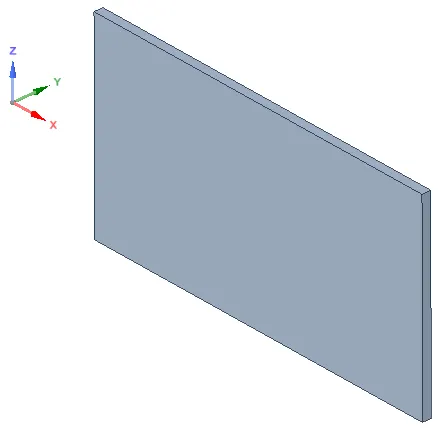
Front-Panel of the housing:

Before simplification After Level 0 (bounding box) simplification

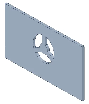
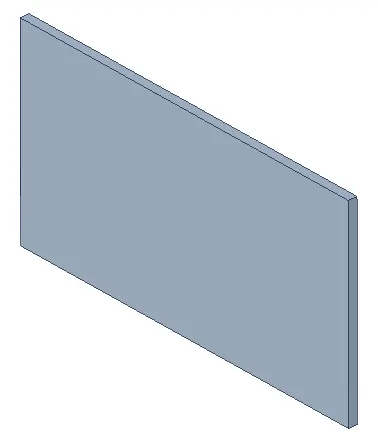
The images attached below show the simplified model.

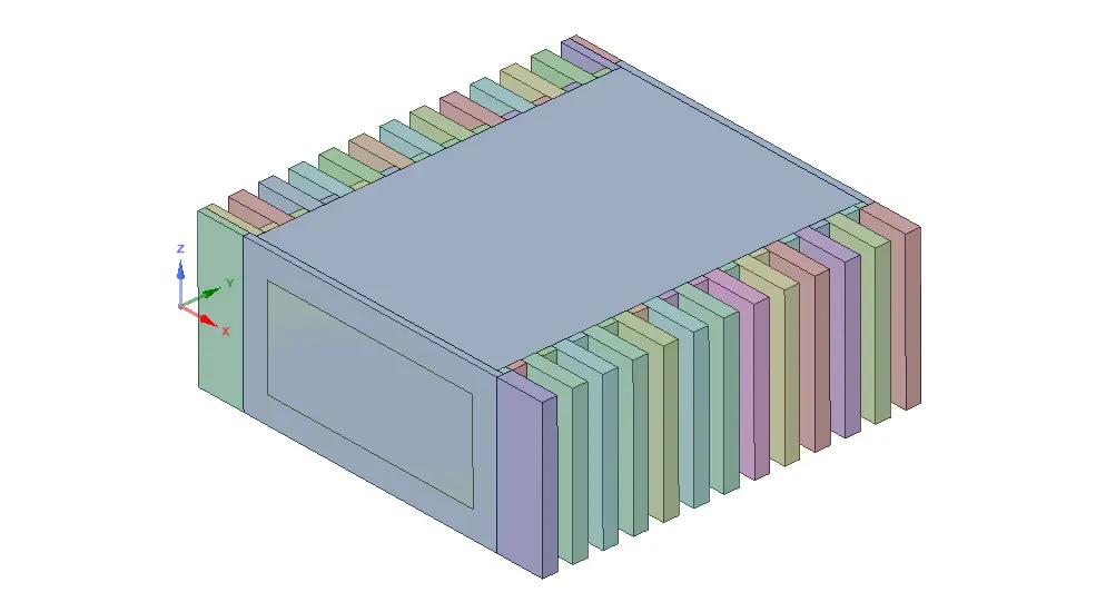
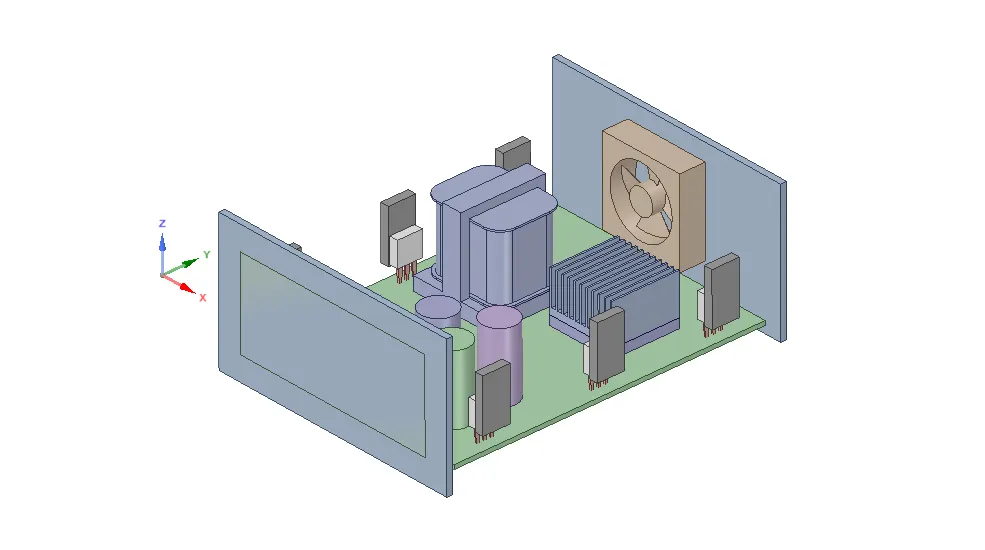
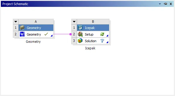
A suitable workflow is created in ANSYS Workbench in order to import the simplified model shown above. The image attached below shows the workflow.

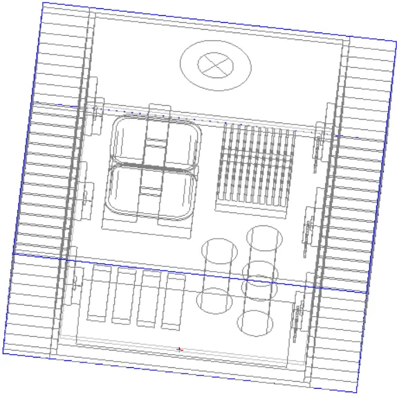
The images attached below show the model in Icepak graphics window.

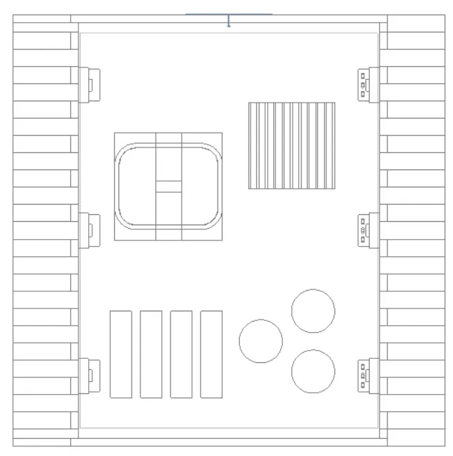
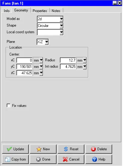
In order to simplify the model even further, the 3-D fan imported from ANSYS SpaceClaim is replaced with a 2-D Icepak fan which serves the same purpose. The image attached below shows the settings applied in the "Geometry" tab to define the fan.

In order to reduce the overall mesh count by preventing mesh bleeding, non-conformal meshing technique is applied. Assemblies are defined around key objects that affect the flow and/or temperature field. The image attached below shows the assemblies with appropriate slack settings.

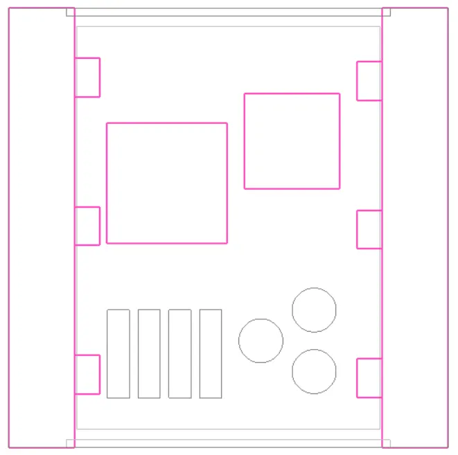
All the assemblies shown above employ the global mesh control settings except the assembly defined around the CAD object "Coil". In order to capture the geometry of the CAD object ("Coil") accurately the following settings are applied for the mesh within the assembly:

1. Mesh type: Mesher-HD

2. Max element size

2.1. X: 1.5 mm

2.2. Y: 1.5 mm

2.3. Z: 0.5 mm

3. Set uniform mesh params: Enabled

3.1. Use average: Enabled

4. Allow multi-level meshing: Enabled

4.1. Max Levels: 2

Meshing:

The computational domain is discretized using Hexa unstrucutred mesh with the following settings:

1. Max element size

1.1. X: 6.35005 mm

1.2. Y: 6.35005 mm

1.3. Z: 2.54005 mm

2. Mesh parameters: Normal

3. Min elements in gap: 3

4. Min elements on edge: 2

5. Max size ratio: 2

6. Mesh assemblies separately: Enabled

For the current model, the mesh is locally refined within the objects "BGA" and "BGA-Heat-Sink", and the assembly defined around the CAD object "Coil" using per-object meshing parameters.

The generated mesh yields 390125 elements and 455388 nodes. The images attached below show the computational mesh along different planes.

1. Z planes through center

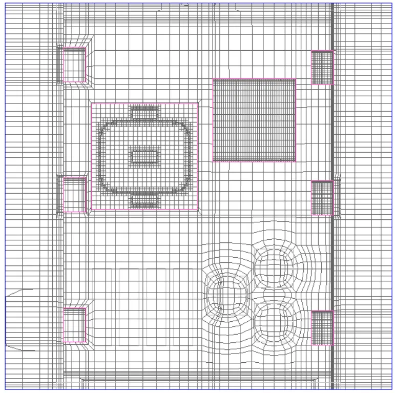
2. Y planes through center

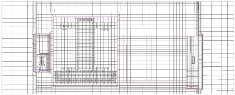
3. X planes through center

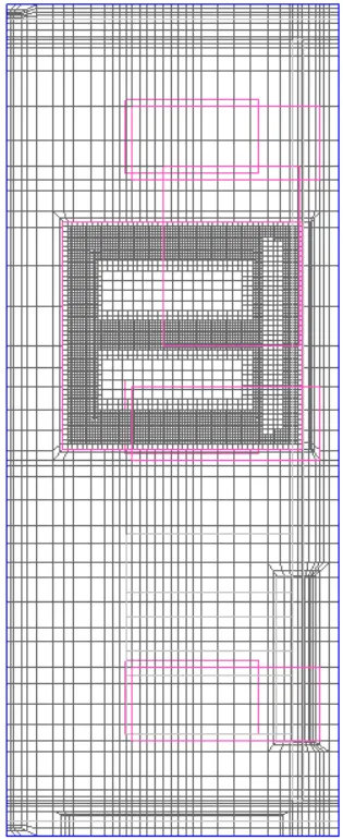
The images attached below show the volume mesh for different objects.

1. BGA

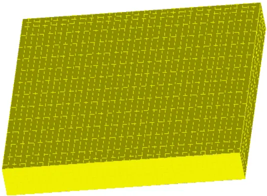
2. BGA-Heat-Sink

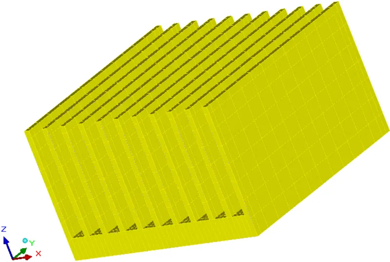
3. Coil (CAD object)

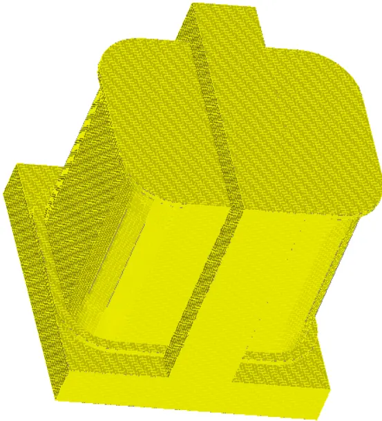
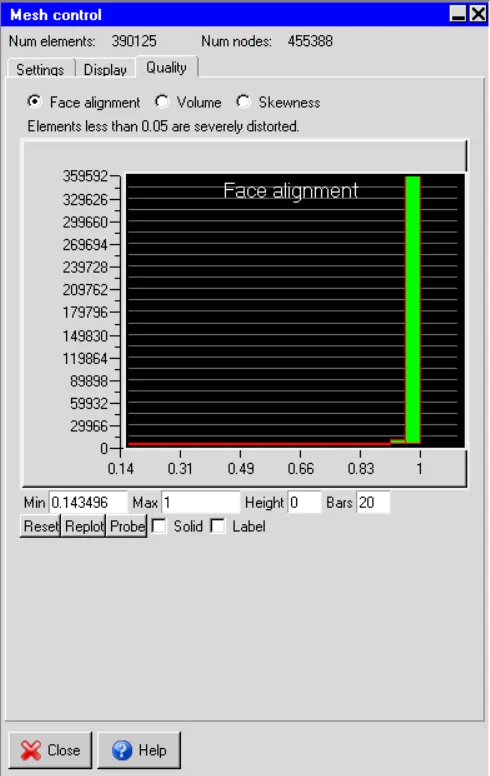
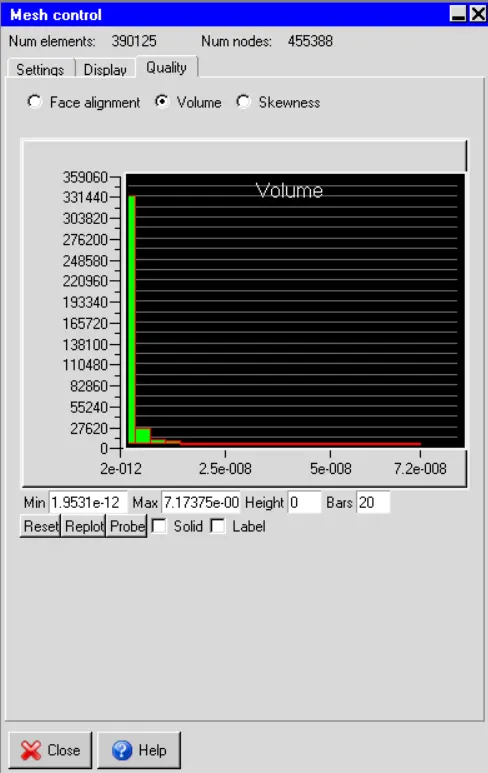
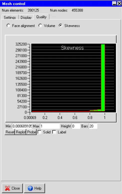
Visually the mesh appears to be fine. The images attached below show the histograms with number of elements plotted along the X-axis and quality measures along the Y-axis.

1. Face alignment

2. Volume

3. Skewness

Solver:

The three dimensional steady-state Navier-Stokes equations for the model are solved within the computational domain for flow and temperature fields, using the Fluent solver available in ANSYS Icepak. The following settings are applied to the solver:

1. Variables solved: Flow (velocity, pressure) and Temperature

2. Radiation: Off

3. Flow regime: Turbulent (Zero equation)

4. Time variation: Steady

5. Solution initialization

5.1. X velocity: 0

5.2. Y velocity: 0

5.3. Z velocity: 0

5.4. Temperature: ambient (20 deg. C)

6. Number of iterations: 200

7. Convergence criteria

7.1. Flow: 1e-6

7.2. Energy: 1e-7

7.3. Joule heating: 1e-7

8. Configuration: Parallel

9. Number of processors: 4

10. GPU computing: Enabled

11. Number of GPUs: 1

12. Precision: Double

The BGA and six dies in the model are assigned a total constant power of 30 W and 2.5 W each, respectively. Hence the total power generated by the model is 45 W. The fan is assigned a fixed volumetric flow rate of 10 cfm.

Results:

In this section, the simulation results are discussed.

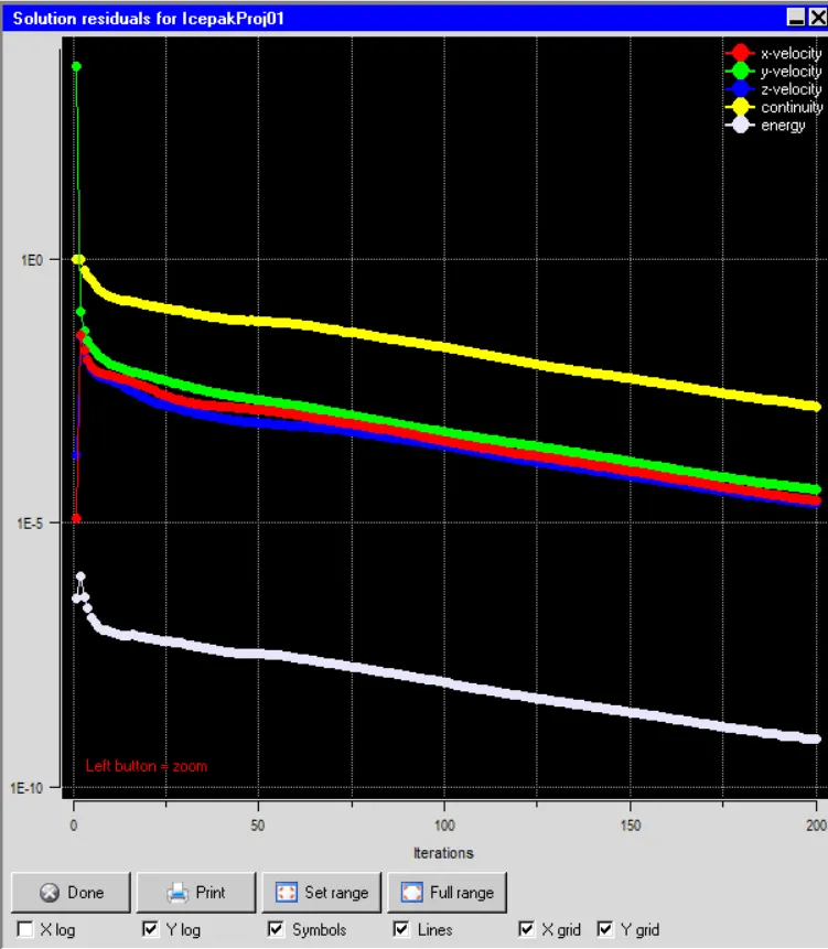
1. Residuals

The residuals for the following equations are plotted against the number of iterations:

i. Continuity equation

ii. X-Momentum equation

iii. Y-Momentum equation

iv. Z-Momentum equation

v. Energy equation

The image attached below shows the residuals plotted against the number of iterations.

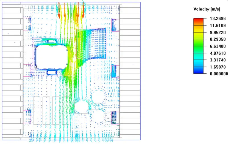
Velocity vectors

The image attached below shows the velocity vectors plotted on the Z-plane through center.

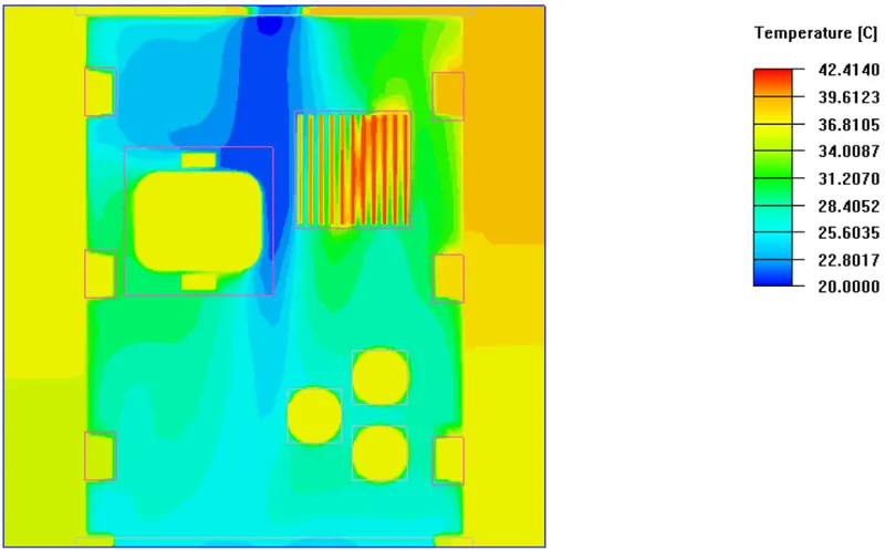
Temperature contours

The image attached below shows the steady-state temperature contours plotted on the Z-plane through center.

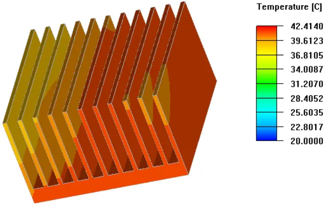
Object face temperature contours:

Conclusion

In the current project, the given CAD model of an electronic enclosure assembly was simplified into an Icepak model using the commands available in ANSYS SpaceClaim. The model was imported into ANSYS Icepak by creating a suitable workflow in ANSYS Workbench. The model was meshed using non-conformal meshing technique and steady state simulation was performed with appropriate solver settings. The following conclusions can be drawn from the simulation results:

1. Both the residual plot and the temperature monitor plot indicated that the solution reached a steady state after 200 iterations.

2. The BGA attains the maximum steady-state temperature (42 deg. C) out of all the assembly components.