Week 5: Prandtl Meyer Shock problem
Aim: To simulate the Prandtl-Meyer Shock flow in Converge CFD.
shock wave:
A shock wave is a type of propagating disturbance that moves faster than the local speed of sound in the medium. Like an ordinary wave, a shock wave carries energy and can propagate through a medium but is characterized by an abrupt, nearly discontinuous, change in pressure, temperature, and density of the medium.
Shock flow boundary conditions:
1. Dirichlet boundary condition
In the Dirichlet boundary condition, the value of the function is given at the boundary.
y(x)=f(x)">y(x)=f(x)
2. Neumann boundary condition
In the Neumann boundary condition, the value of a normal derivative of the function is specified.
∂y/∂n=f(x)
3. Robin boundary condition
It is a weighted combination of the Dirichlet boundary condition and the Neumann boundary condition.
c1y+c2(∂y/∂n)=f
Where C1 and C2 are constants.
4. Mixed boundary conditions
In mixed boundary conditions, the solution of the given equation is required to satisfy different boundary conditions on disjoint parts of the boundary of the domain where the condition is stated.
4. Why do we use Neumann BC at Outlet?
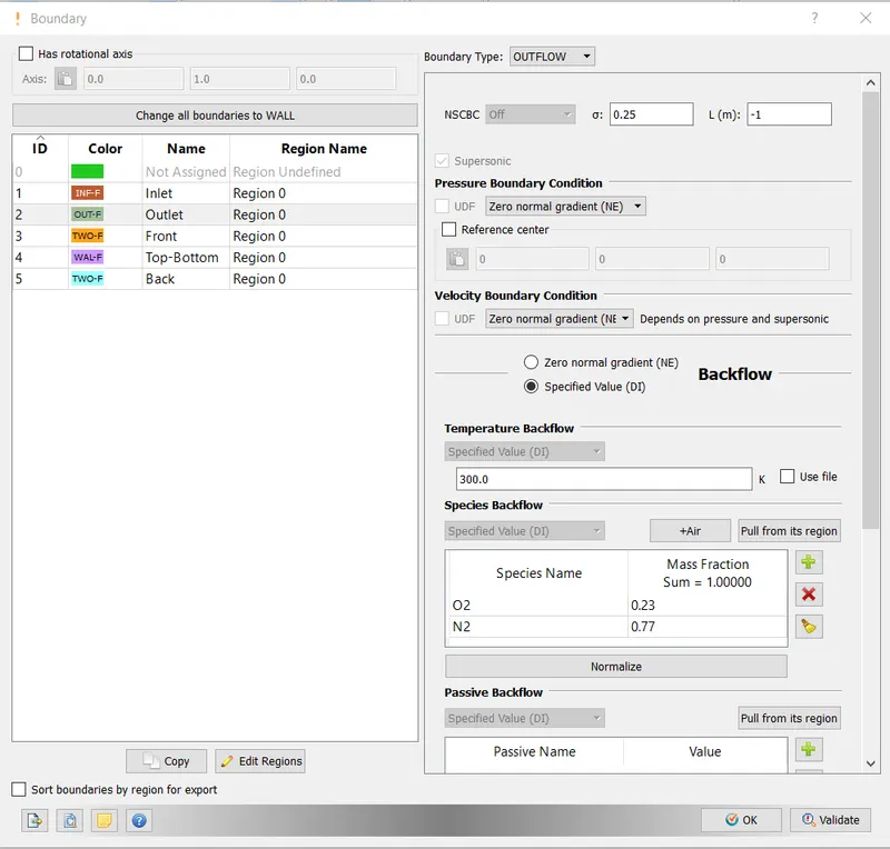
For a supersonic outlet, the characteristic curves propagate outside the domain, along with the streamline. Hence the values of the variable need to be floated, i.e. we calculate the values using linear extrapolation. Hence, we have used Zero normal gradient as the boundary condition for pressure and velocity.
5. Prandtl Meyer Shock
When an object moves faster than the speed of sound, and there is an abrupt decrease in the flow area, shock waves are generated. If the flow area increases, however, a different flow phenomenon is observed. If the increase is abrupt, we encounter a centered expansion fan. There are some marked differences between shock waves and expansion fans.
Across a shock wave, the Mach number decreases, the static pressure increases, and there is a loss of total pressure because the process is irreversible. As the flow across a shock is highly irreversible it cannot be approximated as isentropic. Through an expansion fan, the Mach number increases, the static pressure decreases, and the total pressure remain constant. Expansion fans are isentropic.
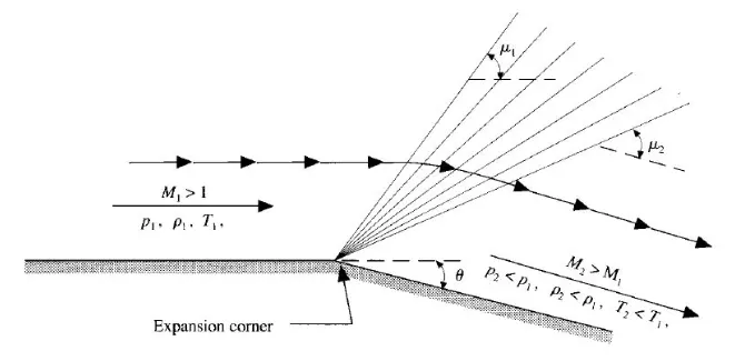
A Prandtl-Meyer expansion wave centered at the point of expansion corner is illustrated in the figure above. An expansion wave which is made up of several Mach waves fans out from the corner. The leading edge of the expansion fan makes an angle of μ1">μ1 with the upstream flow direction and the trailing edge of the wave makes an angle μ2">μ2with respect to the downstream flow direction. These angles are called Mach angles and are defined as,

Where M1 and M2 are upstream and downstream Mach numbers respectively. As the flow passes through the expansion wave, the Mach number increases, and pressure, temperature, and density decrease. The flow upstream and downstream is always parallel to the wall.
Types of Shock Waves:
1. Moving Shock- Consists of a shock propagating into a stationary medium
2. Detonation Wave- A detonation wave is essentially a shock supported by a trailing exothermic reaction. It involves a wave traveling through a highly combustible or chemically unstable medium, such as an oxygen-methane mixture or a high explosive. The chemical reaction of the medium occurs following the shock wave, and the chemical energy of the reaction drives the wave forward.
3. Bow Shock- These shocks are curved and form a small distance in front of the body. Directly in front of the body, they stand at 90 degrees to the oncoming flow and then curve around the body.
4. Attached Shock-These shocks appear as attached to the tip of sharp bodies moving at supersonic speed.
Typical Boundary conditions applicable to Computational Fluid Dynamics problems:
Given below are the typical boundary conditions applied to CFD problems:
i. Wall: The wall type boundary condition can be imposed in the following ways:
(a) Solid wall: A solid wall can have a slip or no-slip boundary conditions depending on whether the flow is inviscid or viscous respectively.
- Slip: v=0 (No penetration boundary condition) : applicable to inviscid flows
- No-slip: u=v=w=0 : applicable to viscous flows
(b) Moving wall: For a moving wall, the fluid in contact attains the same velocity as the wall.
(c) Porous wall: For a porous wall generally the pressure gradient through it is provided.
ii. Far-field: The far-field type boundary condition can be imposed in the following ways:
(a) Inlet/Inflow: Generally freestream conditions are applied under Inlet/Inflow type boundary conditions.
u=U∞;p=P∞
(b) Outlet/Outflow: The following boundary conditions are generally applied under Outlet/Outflow type boundary condition:
- Freestream
- Prescribed pressure
- Pressure extrapolated from the interior (Neumann)
iii. Symmetry: The symmetry type boundary condition implies the following:
- No flow across the boundary
- No scalar flux across the boundary
iv. Periodic: The periodic type boundary condition implies that the flux of all variables at the periodic boundaries are repeated.
The aim of the simulation is to study the following:
(a) Effect of sub-grid scale (SGS) parameter on the expansion fan and cell count.
(b) Effect of initial conditions (specifical velocity) on the results.
1. Geometry
The geometry in STL format was imported into CONVERGE for analysis.
The figure given below shows the geometry of the problem.
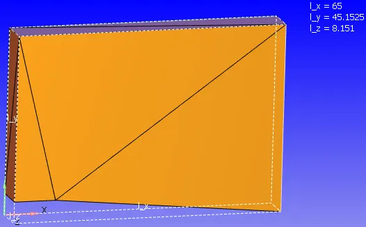
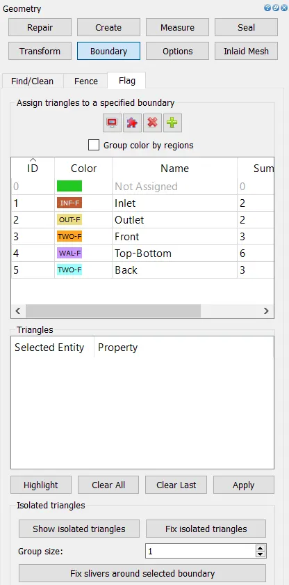
Creation of Boundaries: In the geometry which is created above, boundaries such as inflow, outflow, top and bottom walls, front and back faces are labeled.
Checking Orientation of Normals: The orientation of Normals was checked to ensure all the normals are pointing inwards. This was done using the Normal Toggle
Finally, a Diagnosis check was run to ensure no errors in the geometry.
Case Setup:-
Application Type:- This was set to Time-based
Materials:- This was set to Air
i) Gas Simulation: Default properties were retained
ii) Global Transport Parameters:- Default properties retained
iii) Species: Add the O2 and N2.
Simulation Parameters:-
Run Parameters:- Steady-state solver was used.
A simulation model was set to Full Hydrodynamic.
Gas Flow solver set to Compressible
Steady State Monitor:- Minimum no of cycles for to be executed for Steady-state solver -500
Monitor Start Delay, cyc :- 200
Sample size cyc :- 100
Simulation Time Parameters:- The parameters were set as displayed below. The simulation was run for 25000 cycles. Max CFL limit set to 1.0
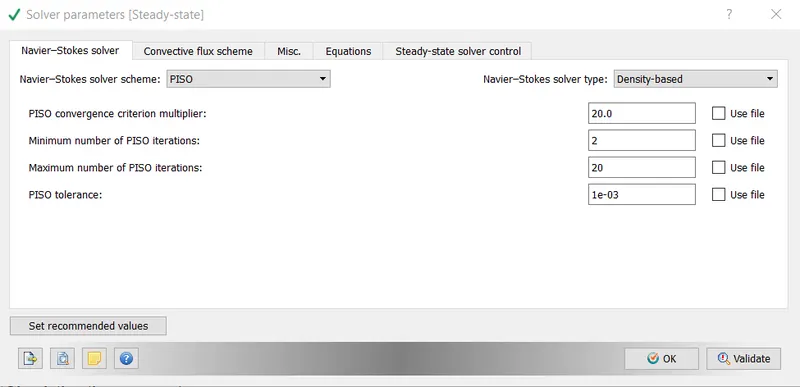
Solver Parameters:- A Pressure based PISO solver was used, Maximum Convection CFL limit set to 0.8
Boundary:
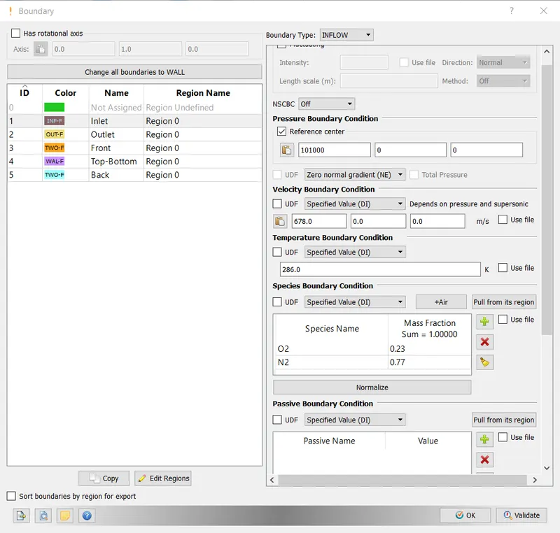
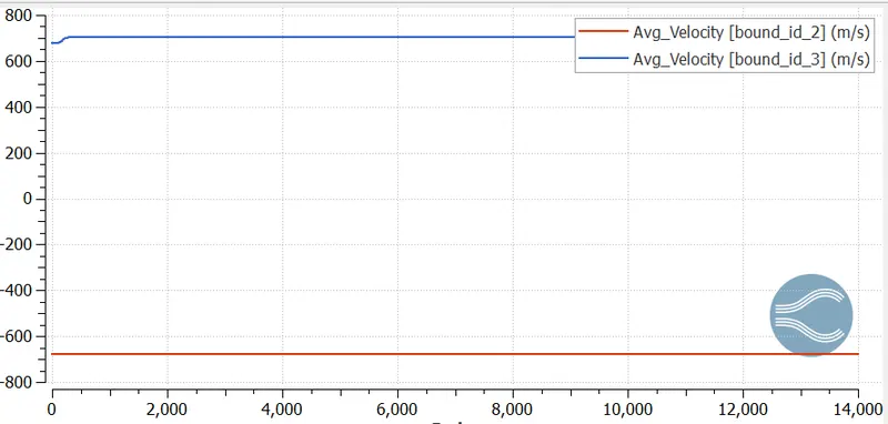
Inlet: Since it’s a supersonic flow at the inlet we should assign Dirichlet boundary conditions for all parameters like Pressure, Velocity, and Temperature. So, We can give Static pressure= 101000 Pa, Velocity=678m/s and Temperature=286k
Outlet: At the outlet, we should assign Neumann boundary conditions for all parameters like Pressure, Velocity, and Temperature. So, We can give a Zero normal gradient for all the parameters.
Top-Bottom wall:
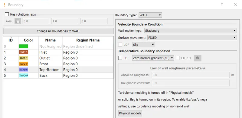
Since the supersonic flow is inviscid in nature(the viscous effect is negligible) we can assume the Slip condition at the wall.
Front-Back: 2D Wall
Reason: The 2D planar assumption is used because the flow gradients along the z-direction are negligible when compared to the other two directions. By reducing the model to 2D, the Prandtl Meyer can be simulated and analyzed cost-effectively compared to a full 3D model.
Initial condition and events
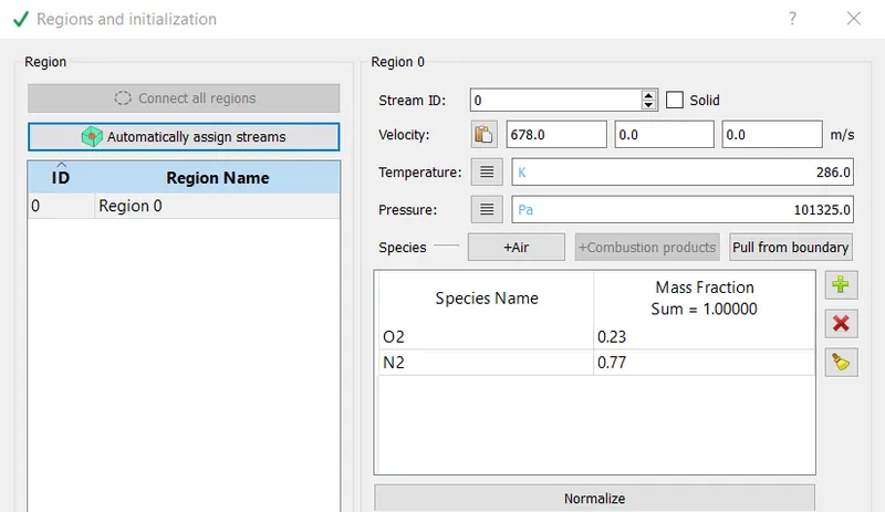
The created geometry was selected as the Volumetric Region. The velocity was set to 678m/s
Turbulence Modelling: No need for the Turbulence model.
Reason: In our simulation, we don't have to use Turbulence modeling since there is no Reynolds stress because the flow is inviscid.
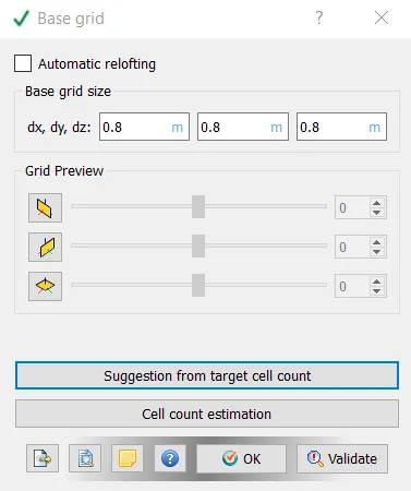
Grid Control:- Base Grid. Here the size of the mesh is entered.
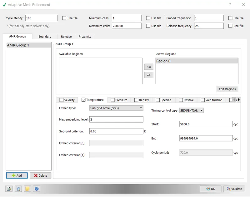
Adaptive Mesh Refinement was also enabled. A temperature-based adaptive mesh refinement technique was used in which the curvature of temperature is monitored. Whenever the curvature of temperature is greater than a particular value the mesh would be refined. It can be thought of as sub-grid scale temperature.
In the below snapshot, we see that the sub-grid scale criterion is set to 0.05K. This implies that whenever the temperature difference is greater than 0.05 K, AMR will refine. The maximum embedding level is set to 2, this means that there will be two layers of refinement. Converge uses an octree data structure. In this data structure, the grid size can be calculated by the given formula
In this case, the base grid size is 0.08. The smallest grid size will be 0.08/(2^2) which means the smallest grid size will be 0.02.
A computational grid with the following features is used for all cases:
i. Base grid: dx=dy=dz=0.8m
ii. Adaptive Mesh Refinement (AMR):
Minimum cells: 1
Maximum cells: 200000
Temperature Sub-Grid Scale (SGS) criterion: 0.05K (Case 1 and Case 4); 0.1K (Case 2); 0.2K (Case 3)
Maximum embedding level: 2
Timing control type: SEQUENTIAL
Start: 5000 cycles
End: 999999999 cycles
The figure shown below shows the base grid for all cases.
Output/Post Processing:- The variables that we intend to see during post-processing are selected. In this case, Density, Pressure, Temperature, and Velocity were selected.
Here 3 cases are set and those are for subsonic and supersonic flow and for low and high SGS parameters.
Now export all input files: Click on files > Export > Export input files > choose the path and select all files and press ok.
Run the simulation and post-convert the files: Copy and paste the mpiexec.exe file and converge.exe file to the folder in which the input files are exported to run the simulation in Cygwin. Copy the post_convert_30_msmpi_64.exe file and paste it into the output folder. Now open Cygwin and go to the output folder and type mpiexec.exe -n 4 post_convert_30_msmpi_64.exe > enter the case name(as case1) > select file type as Paraview VTK in-line binary format > type all for files and cell variables and click enter (or) we can convert those files in converge studio.
Post-processing the files:
To post-process the files lanch paraview and open the file location as case1 which is saved in output > case1 .. vtm (this is a group file which is formed during post-converting the files) > click on apply > create a slice along the z-axis.
Results:
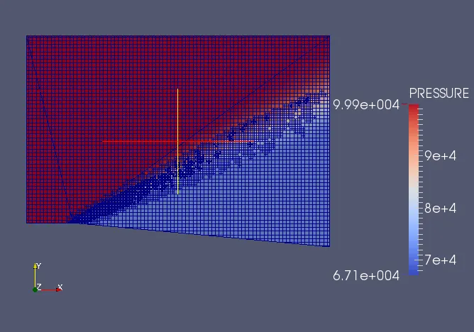
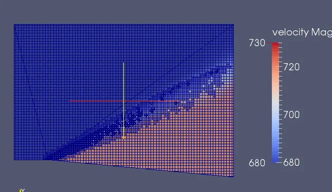
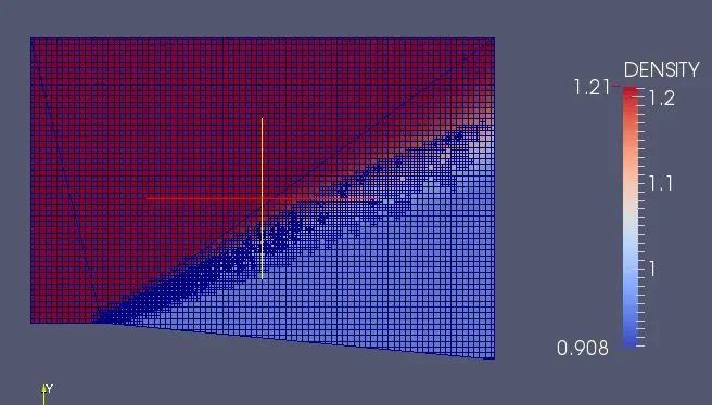
Case 1: Countors for Supersonic flow
Plots:
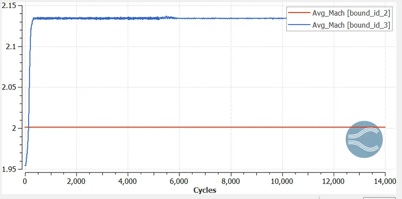
Mach number:
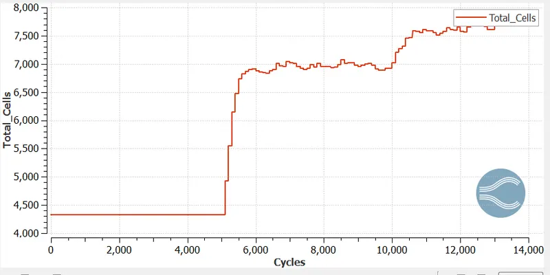
Total cells:
velocity:
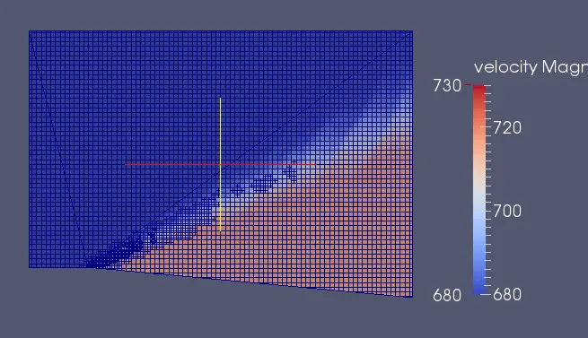
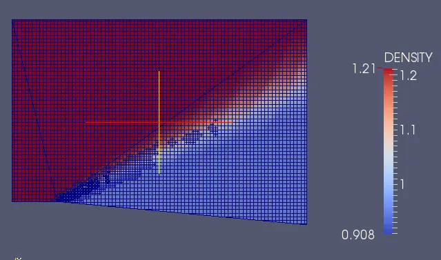
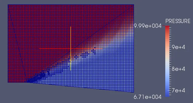
Case 2: Countors for Supersonic flow with low SGS parameter(0.1)
Plots:
Pressure:
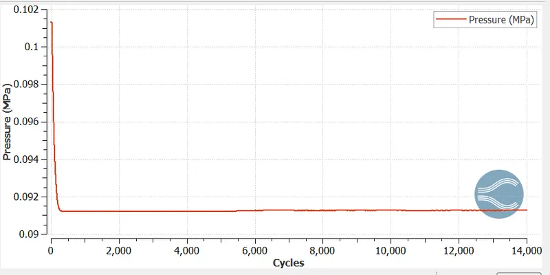
Mach number:
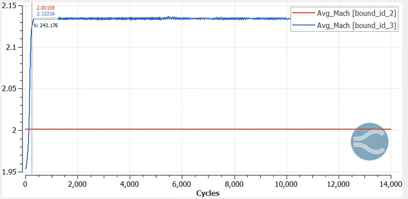
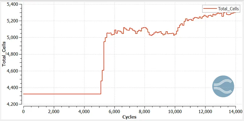
Total cells:
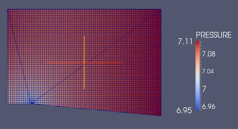
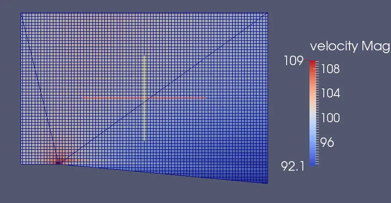
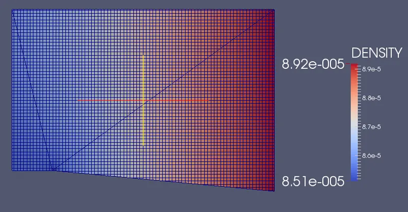
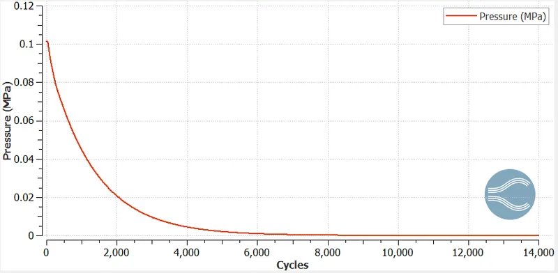
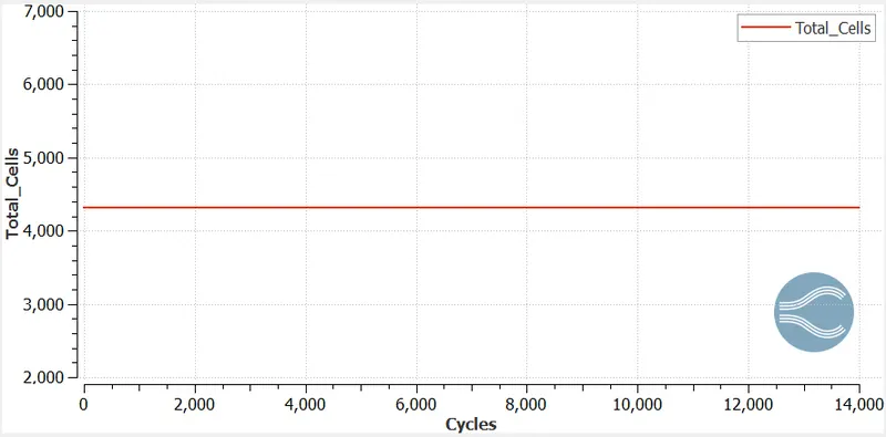
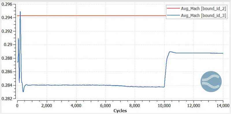
Case 3: Countors for Subsonic flow(velocity=100, SGS = 0.05)
Plots:
Pressure:
Total cells:
Mach number:
Animation link:
Case1:
Case2:
Case3:
Effect on SGS parameter on shock location and total cell count:
- From the above results, the SGS parameter decreases the total cell count increases and there is more formation of cells around the shock wave.
- For a high SGS parameter, the mesh refinement area is very small like in case-2.
Conclusion:
- In supersonic flow, the Prandtl-Meyer expansion fan is clearly visible and the mesh refinement is also visible in the shock region.
- Whereas in the subsonic flow, the Prandtl-Meyer expansion fan is not visible at all and the mesh refinement is also not visible. This is due to no shock waves(sudden change in pressure, temperature, velocity, and density).
- As the SGS parameter decreases, the total cell count increases, and the mesh refinement area spread from the sharp edge to the outlet boundary. If the SGS parameter increases, the mesh refinement area is very small and it doesn't spread to the outer boundary.