Week 6: Conjugate Heat Transfer Simulation
Aim:-
To simulate the Conjugate Heat Transfer over pipe using Super- Cycling in CONVERGE and determine Y+.
Objective:-
In the current project conjugate heat transfer analysis of flow through a circular pipe is performed using CONVERGE CFD, with the following objectives:
i. To study the effect of grid size on the simulation results: The following three grid sizes are used:
(a) dx=dy=dz=0.004m
(b) dx=dy=dz=0.003m
(c) dx=dy=dz=0.002m
The results of this study are discussed in section 1 of Results and discussions.
ii. To study the effect of super-cycle stage interval on the simulation results: The following four intervals are used for the super-cycle stage:
(a) 0.01s
(b) 0.02s
(c) 0.03s
(d) 0.05s
The results of this study are discussed in section 2 of Results and discussions.
Theory:-
Conjugate Heat Transfer:-
- Conjuate Heat Transfer correspond with the combination of heat transfer in solid and heat transfer in fluid.
- In solid, conduction often domain whereas in fluid convection usually domain.
- Conjugate heat transfer is observed in many situation. For egs, heat sinks are optimized to combined heat transfer by conduction in the heat sink with the convection in the surrounding field.
Super-Cycling Method:-
- In Super-Cycling method, the fluid solver working on convection problem is paused for a small time period allowing the solid state conduction solver catch up, this method significantly reduce the number of cycle and simulation time.
Output Y + :-
- Wall function are useful in telling the solver how to approch the solution near a wall. These used to predict near wall result accurately even at coarse grid.
- The Y + value is a non-dimensional term that can be used to understand how coarse grid are fine, this can then be used to determine if wall function need to be used or not.
Geometry:-
The geometry used for performing simulations consists of a cylindrical pipe having the following dimensions:
Thickness=0.005m
Length=0.2m
Creation of geometry. A concentric pipe with internal diameter of 0.03m and external diameter of 0.04m was created for the purpose of the analysis.
The figure given below shows the geometry:
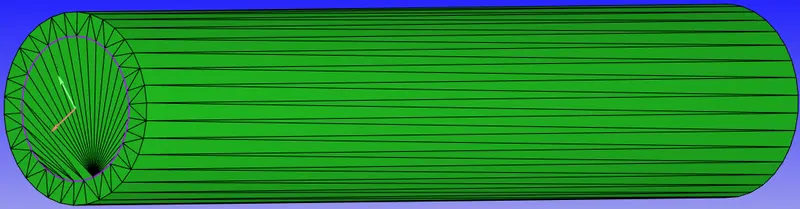
After creating the geometry, a diagnosis check was performed in with intersection errors were noticed. These were rectified by selecting the Repair option under Geometry. The Front two faces and the rear faces were selected and deleted.
Boundaries were created as listed below
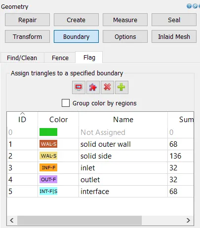
The direction of the normals were found to be incorrect and were rectified to ensure the normals are pointing inwards to the direction of fluid flow.
After completion of the above steps a diagnosis check was again performed. Non manifold edges were observed and this was as a result of interface between solid and fluid.
Case Setup:-
i) Materials:- Gas simulation, Solid Simulation and Species were selected.
Gas Simulation:- Default retained
Solid Simulation:- The Material used was Aluminium
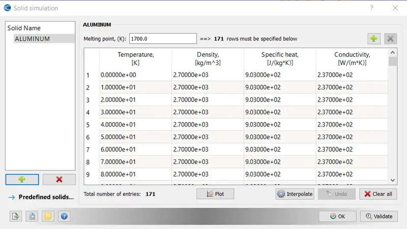
Global Transport Parameters:- Default values retained
Species:-
a) Gas:- O2 and N2
b) Solid:- Aluminium
ii) Simulation Parameters:
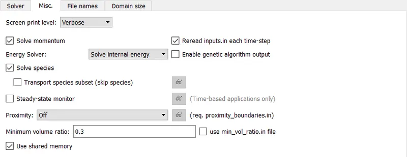
Run Parameters:- Simulation set to Transient.
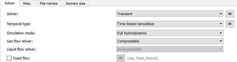
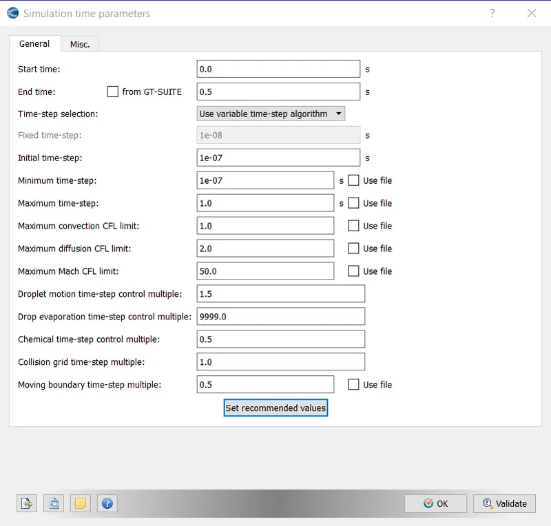
Simulation Time Parameters:- Values set as shown below.
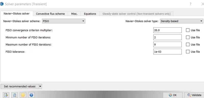
Solver Parameters (Transient):- Defaults value retained
iii)Boundary:-
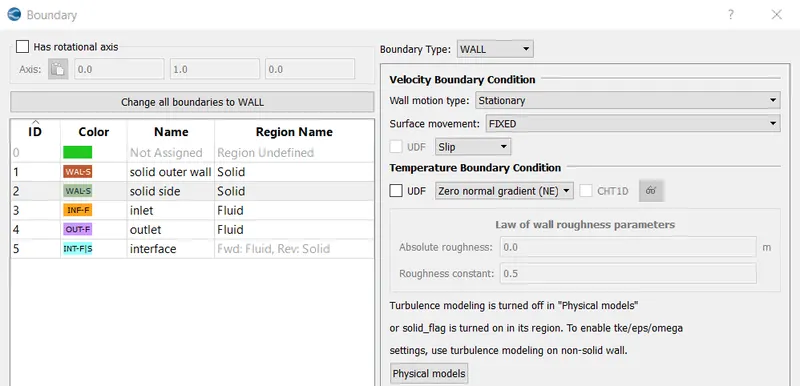
Solid Outer Wall:- A Heat Flux of -10000 W/m^2 is introduced. The negative sign indicates that heat flux is flowing into the pipe.
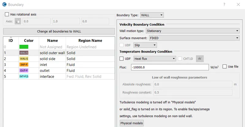
Solid Side:- Wall motion type is set to stationary, surface movement fixed
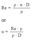
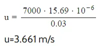
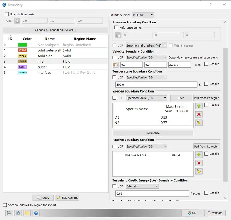
Inlet:- In the problem it is given that the inlet Reynolds number should be 7000. The value of the inlet velocity is computed from the below formula
The value of Kinematic viscosity at 300 K is 15.69 * 10^-6. Also the diameter is taken to be the internal dia of the pipe which is 0.03m/
Outlet:- Pressure Value set to 101325 Pa at the outlet
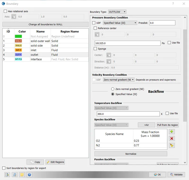
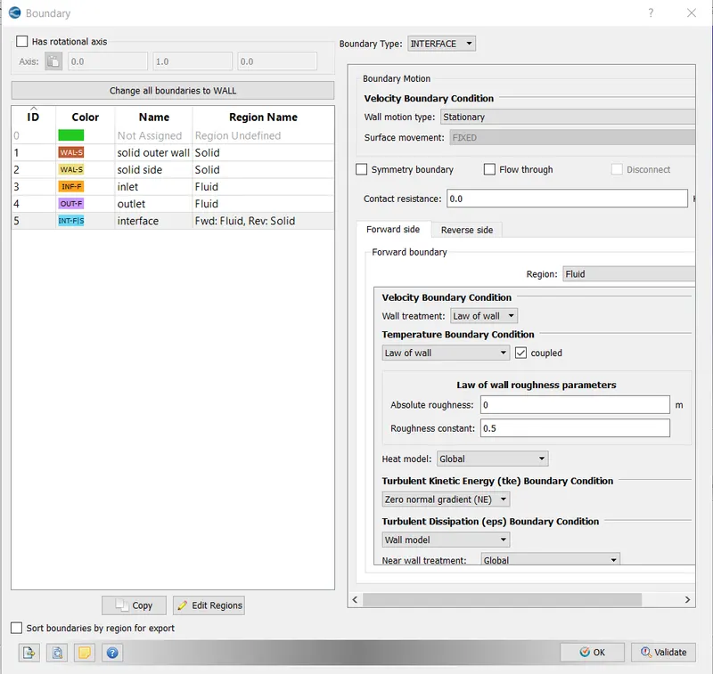
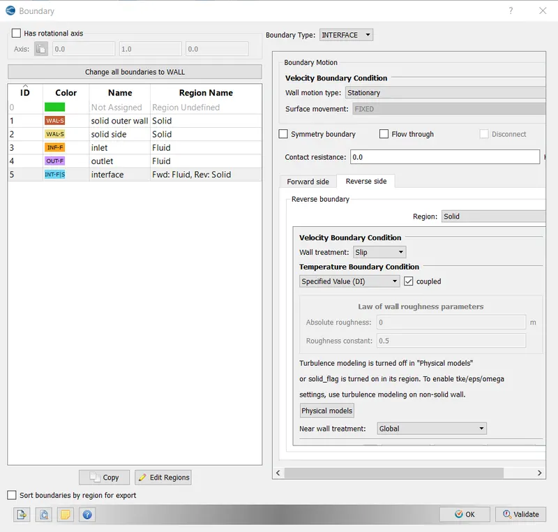
Interface:- The normals on the interface point towards the fluid regionand this is referred to the forward side. The opposite direction which points towards the the solid direction referred to as reverse direction.
Velocity and Temperature boundary condition in forward region set to Law of the Wall
In Reverse region Velocity and temperature set to slip and specified value respectively
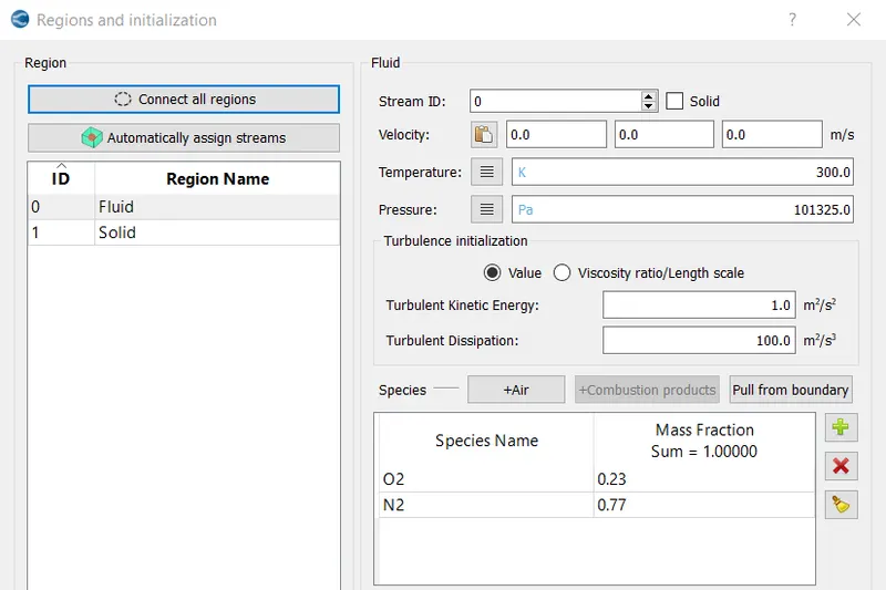
Regions and Initialization:-
i) Fluid Region:- Values set as shown below
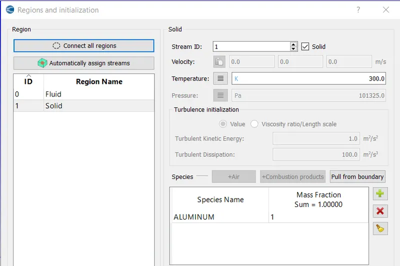
ii) Solid Region:- Stream Id set to 1 and solid box checked
Turbulence Modelling:- k epsilon model is used
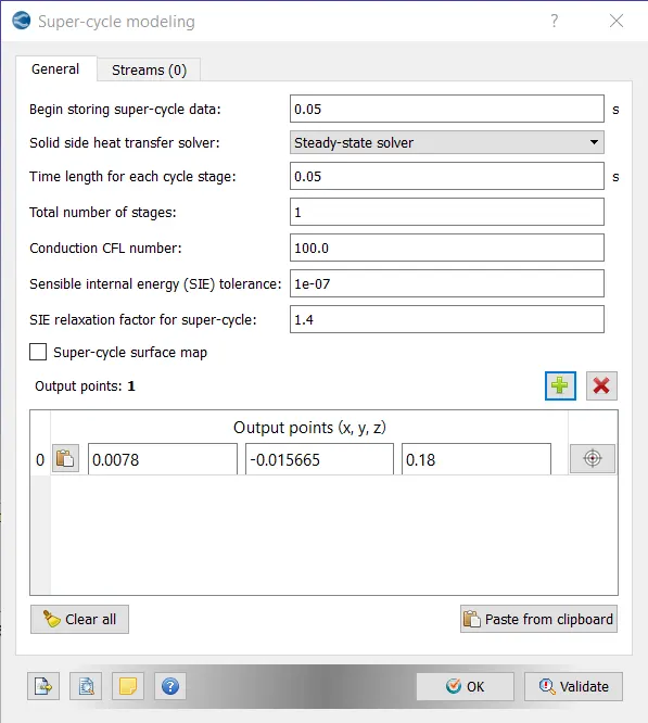
Supercycling was enabled in order to reduce the computational time requried for CHT analysis. A monitor point was created at the outlet. Time length was initially set to 0.05 and then reduced to 0.03,0.02 and 0.01.
Base grid size was set to 0.004, 0.003 and 0.002
In post variable selection, apart from the usual default, wall yplus and heat transfer coefficient was enabled.
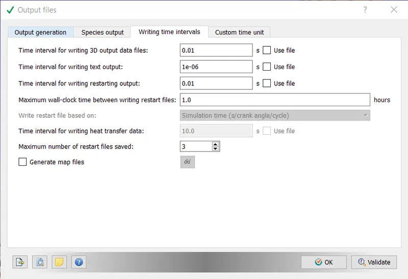
The time intervals for writing output files was set as given below
In order to execute the simulation, the directory in which these input files were stored was accessed in Cygwin and the following command was typed "mpiexec.exe -n 4 converge.exe"
After the Simulation was executed, the results were converted into a form which would be compatible with Paraview. This was done using the post_convert.exe command.
Grid:-
For study i (effect of grid size), three different grid sizes are used:
(a) dx=dy=dz=0.004m
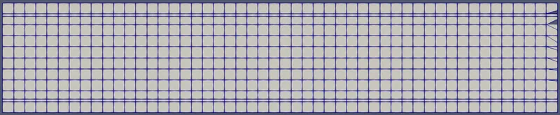
(b) dx=dy=dz=0.003m
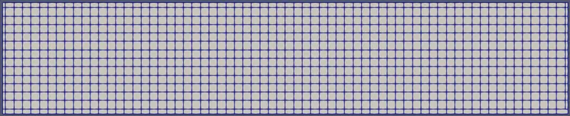
(c) dx=dy=dz=0.002m
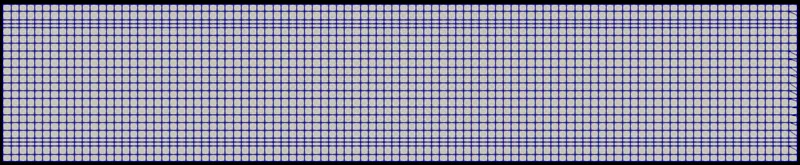
For study ii (effect of super-cycle stage interval), a grid size of dx=dy=dz=0.004m is used.
Results and discussions:-
In this section, the simulation results are discussed. Section 1 deals with the simulation results of study i (Effect of grid size) whereas section 2 deals with the results of study ii (Effect of super-cycle stage interval).
1. Effect of grid size
As mentioned previously, for this study the case is simulated using the following three base grid sizes:
i. dx=dy=dz=0.004m: Mesh 1
ii. dx=dy=dz=0.003m: Mesh 2
iii. dx=dy=dz=0.002m: Mesh 3
1.1. Mean temperature in the solid region
The mean temperature in the solid region is plotted over time for all three meshes.
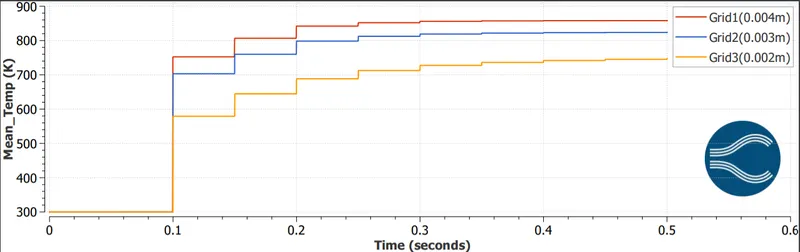
The plot shows that steady-state is achieved for all three meshes. It is also evident that the solution is grid-dependent. The values of mean temperature in the solid region (at 0.5s) for different meshes are as follows:
i. Grid 1 (0.004m): 858.32K
ii. Grid 2 (0.003m): 823.10K
iii. Grid 3 (0.002m): 745.73K
The various super-cycle stages, after 0.05s each, can also be observed on the plot. At each step, the super-cycle data is stored and the steady-state computations are performed for the solid region.
Super-cycle temperature in the solid region:-
The super-cycle temperature at the output point, defined in the solid region, is plotted over time for all three meshes. These plots are generated using the steady-state converged values of temperature at the output point after each super-cycle stage interval.
Note: The super-cycle stage intervals begin after the first time interval, at the end of which the storing of super-cycle data begins.
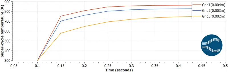
Again, the grid dependence of the solution is quite evident from the plot. The values of super-cycle temperature at the output point for different meshes are as follows:
i. Grid 1 (0.004m): 863.16K
ii. Grid 2 (0.003m): 829.6K
iii. Grid 3 (0.002m): 754.59K
Average fluid temperature at the outlet:-
The average temperature of the fluid region at the outlet is plotted over time for all three meshes.
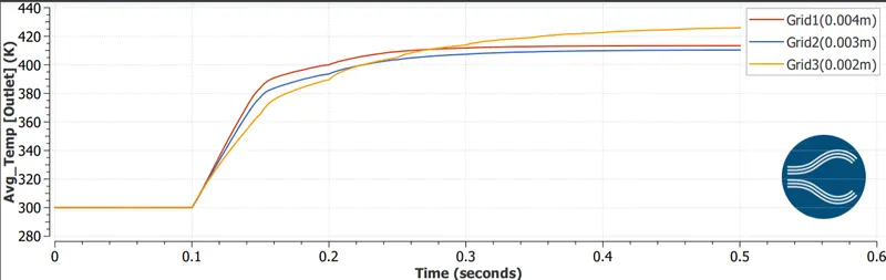
The plot suggests that the average fluid temperature at the outlet converges to nearly equal values for all three meshes.
i. Grid 1 (0.004m): 413.50K
ii. Grid 2 (0.003m): 410.01K
iii. Grid 3 (0.002m): 425.8K
Temperature contours:-
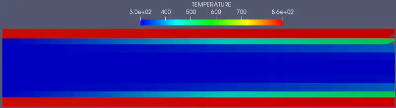
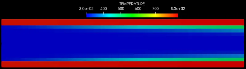
For all three meshes the temperature contours are plotted at a plane passing through the centre of the pipe.
i. Grid 1 (0.004m)
ii. Grid 2 (0.003m)
iii. Grid 3 (0.002m)
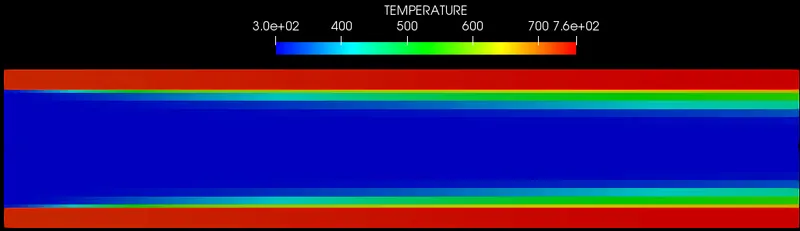
The temperature contour plots show that maximum temperature is achieved by the solid region. It is also evident that the contour plots become smoother with a decrease in grid size. The temperature gradients near the wall, in the fluid, are best resolved by Grid 3 (0.002m). However the solution is still grid-dependent for Grid 3 and hence is not reliable. Also the value of Y+ needs to be checked before employing the Standard Wall Function in the K-ε">K−ε model.
Y+ values:-
In turbulence modeling, Y+ values can be used to decide whether the Standard Wall Function needs to be employed.
For 0
For 10
For Y+>30: The first cell center near the wall lies in the logarithmic layer (turbulent region). For this region, the Standard Wall Function can be employed.
Hence if turbulence model (with Standard Wall Function) is employed for a particular problem, Y+ should be greater than 30. This puts a lower limit on the grid size.
For all three meshes the Y+ contours are plotted at a plane passing through the centre of the pipe.
i. Grid 1 (0.004m)
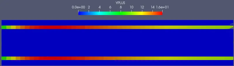
Average Y+ at either wall: 46.24
ii. Grid 2 (0.003m)
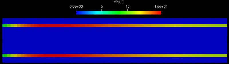
Average Y+ at either wall: 48.25
iii. Grid 3 (0.002m)
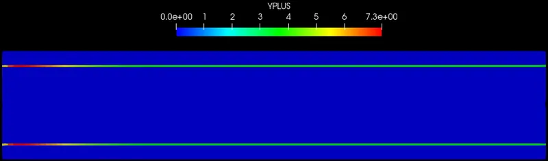
Average Y+ at either wall: 15.49
The average value of Y+ for Grid 3 (0.002m) indicates that the first cell location lies in the buffer layer and since K-ε">K−ε turbulence model (with Standard Wall Function) is employed for the present problem, the results for Grid 3 can't be trusted. Hence the solution of the present problem remains grid-dependent in the region Y+>30.
In order to achieve grid independence, the grid needs to be a lot finer such that Y+ becomes smaller than 10. In such cases, the Standard Wall Function is not required. However simulating the current problem with such grid sizes is computationally quite expensive and hence is not attempted in the current project.
Animation:-
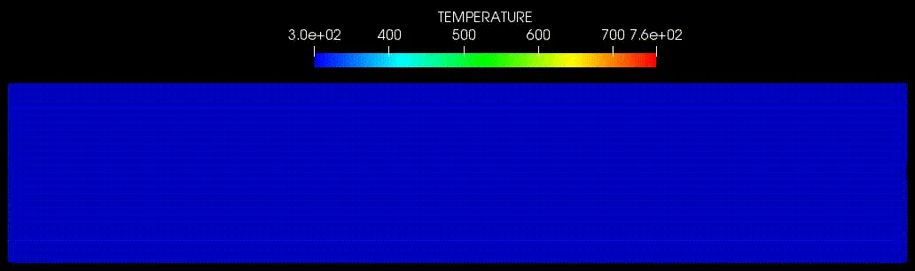
The animations attached below show the evolution of temperature contours with time.
Note: The solution is not time-accurate
i. Grid 1 (0.004m)
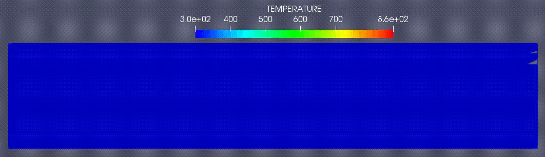
ii. Grid 2 (0.003m)
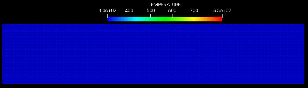
iii. Grid 3 (0.002m)
2.Effect of super-cycle stage interval
For the present study, the following four super-cycle stage intervals are used:
i. SSI 1: 0.01s
ii. SSI 2: 0.02s
iii. SSI 3: 0.03s
iv. SSI 4: 0.05s
For all cases, a grid size of dx=dy=dz=0.004m is adopted.
Mean temperature in the solid region
The mean temperature in the solid region is plotted over time for all three intervals.
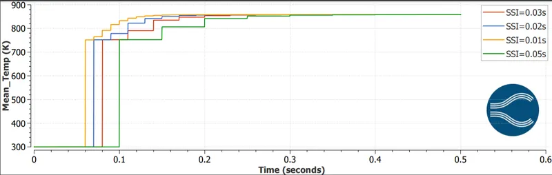
The values of mean temperature in the solid region (at 0.5s) for different super-cycle stage intervals are given below:
i. SSI 1 (0.01s): 858.41K
ii. SSI 2 (0.02s): 858.39K
iii. SSI 3 (0.03s): 858.37K
iv. SSI 4 (0.05s): 858.32K
It can be seen from the plot that for all super-cycle stage intervals the mean temperature in the solid region converges to nearly equal values. The plots also show that with a decrease in super-cycle stage interval the number of super-cycle stages required to achieve steady-state increases.
Super-cycle temperature in the solid region
The super-cycle temperature at the output point, defined in the solid region, is plotted over time for all three intervals.
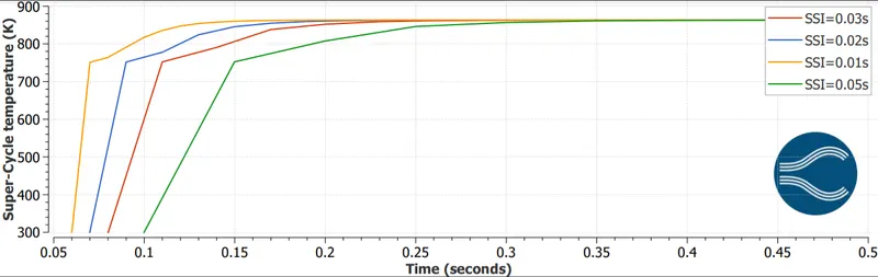
The super-cycle temperature values at the output point for different super-cycle stage intervals are given below:
i. SSI 1 (0.01s): 863.26K
ii. SSI 2 (0.02s): 863.24K
iii. SSI 3 (0.03s): 863.22K
iv. SSI 4 (0.05s): 863.16K
For all super-cycle stage intervals the super-cycle temperature converges to nearly identical values.
Average fluid temperature at the outlet
The average temperature of the fluid region at the outlet is plotted over time for all three intervals.
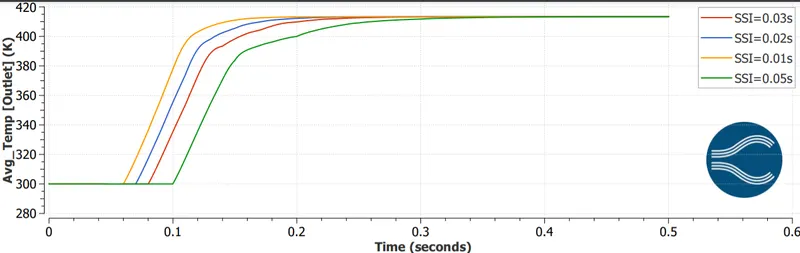
i. SSI 1 (0.01s): 413.53KThe values of average temperature of the fluid region at the outlet for different super-cycle stage intervals are as follows:
ii. SSI 2 (0.02s): 413.53K
iii. SSI 3 (0.03s): 413.52K
iv. SSI 4 (0.05s): 413.50K
For all super-cycle stage intervals the average temperature of the fluid region at the outlet converges to nearly identical values.
Simulation time:-
The table attached below shows the effect of super-cycle stage interval on the simulation time.
| Super-cycle stage interval(s) | Simulation time(s) |
| 0.01 | 426 |
| 0.02 | 437 |
| 0.03 | 457 |
| 0.05 | 522 |
Conclusion:-
The following can be concluded from the simulation results:
i. The solution remains grid-dependent over the three employed grid sizes. For achieving grid independence even smaller grid sizes need to be investigated. However due to limitations on the available computational resources, such a task is not attempted in the current project.
ii. With a decrease in the super-cycle stage interval, the number of super-cycle stages required to achieve steady-state increases.
iii. With an increase in the super-cycle stage interval, the simulation time increases.