Week 5 - Rayleigh Taylor Instability
Rayleigh Taylor Instability
Objectives:
1. To develop a numerical case set-up for Rayleigh-Taylor instability problem in Ansys Fluent.
2. To conduct grid dependency test to understand the variation in RT instabilites.
3. To understand the effect on RT instabilities due to variation in Atwood number.
INTRODUCTION
The Rayleigh–Taylor instability, is an instability of an interface between two fluids of different densities which occurs when the lighter fluid is pushing the heavier fluid. It is a dynamic process where in system tries to reduce its combined potential energy.
Let us consider two completely plane-parallel layers of immisible fluid, the more dense on top of the less dense one and both subject to the Earth's gravity. The equilibrium here is unstable to any perturbations or disturbances of the interface: if a parcel of heavier fluid is displaced downward with an equal volume of lighter fluid displaced upwards, the potential energy of the configuration is lower than the initial state. Thus the disturbance will grow and lead to a further release of potential energy, as the more dense material moves down under the (effective) gravitational field, and the less dense material is further displaced upwards.
Rayleigh-Taylor instability is a type of hydrodynamic instability which arises due to density differences between 2 fluids that are placed one on top of the other. The fluid on top is denser than the bottom fluid. This creates an instability at the interface. If the lighter fluid maintains sufficiient pressure, then the interface will remain undisturbed.
But a slightest disturbance can cause the interface to become unstable, after which the heavier fluid moves, accelerating with gravity and lighter fluid rises as bubbles into the heavier fluid due to buoyancy forces.
For the base case simulations, water and air are considered. The major forces that contribute towards this instability are hydrodynamic pressure and the buoyancy force.
Types of Instability and practical CFD models based on mathematical analysis of RT waves:
* Ritchmyer-Meshkov instability:
The Richtmyer-Meshkov instability aries when a shock wave interact with an interface separating two different fluids. It combines compressible phenomena, such as shock interaction and refraction, with hydrodynamic instability,including nonlinear growth and subsequent transition to turbulance,across a wide range of Mach numbers.
* Plateau-Rayleigh instability:
The Plateau–Rayleigh instability, often just called the Rayleigh instability, explains why and how a falling stream of fluid breaks up into smaller packets with the same volume but less surface area. It is related to the Rayleigh-Taylor Instability and is part of a greater branch of fluid dynamics concerned with fluid thtread breakup. This fluid instability is exploited in the design of a particular type of ink jet technology whereby a jet of liquid is perturbed into a steady stream of droplets.
* Kelvin-Helmholtz instability:
can occurs when there is velocity shear in a single continous fluid, or additionally where there is a velocity difference across the interface between two fluids. An example is a wind blowing over water. The instability manifests in waves on the waves on the water surface. More generally, clouds, the ocean,Saturn's bands, and the sun's corona show this instability.
Practical CFD Models:
* SPH method (Smoother particle hydrodynamics)
Smoothed-particle hydrodynamics (SPH) is a computational method used for simulating the mechanics of continuum media, such as solid mechanics and fluid flows. Smoothed-particle hydrodynamics is being increasingly used to model fluid motion as well. This is due to several benefits over traditional grid-based techiques.First, SPH guaranteees conservation of mass without extra computation since the particles themselves represent mass. Second, SPH computes pressure from weighted contributions of neighboring particles rather than by solving linear systems of equations. Finally, unlike grid-based techique, which must track fluid boundaries, SPH creates a free surface for two-phase interacting fluids directly since the particles represent the denser fluid and empty space represents the lighter fluid.
* Single Fluid Model
A typical approach used for the analysis of two-phase flows is a mixture model, i.e the individual fluid phases are assumed to behave as a flowing mixture described in terms of the mixture properties. The applied single-fluid model is afive equation model consisting of the mass, momentum and energy equations for a vapor/loquid mixture, and two equations describing the formation and growth of the liquid phase.
* Two Fluid Model
In the two-fluid model, separate sets of the governing equation for the vapor and liquid phases have been usewd. The interaction between the droplets and the heat exchange between the liquid phase and the solid boundary are not modelled here as well. Additionally, the velocity slip between vapor and the liquid phase is in this model taken into account.
Approach:
To simulate the instability, the conditions and values considered in terms of geometrical and computational aspects are mentioned below.
The fluids are assumed as:
- water
- Air
Geometrical aspects:
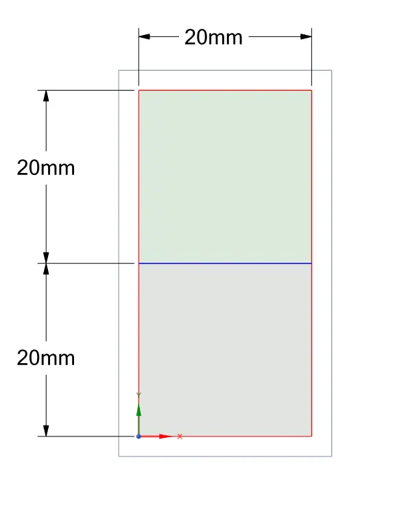
- Two square blocks of size (20mm*20mm)are used to build the required geometry.
- Share topology option in Spaceclaim is used to connect the interface between 2 blocks.
CASE-1
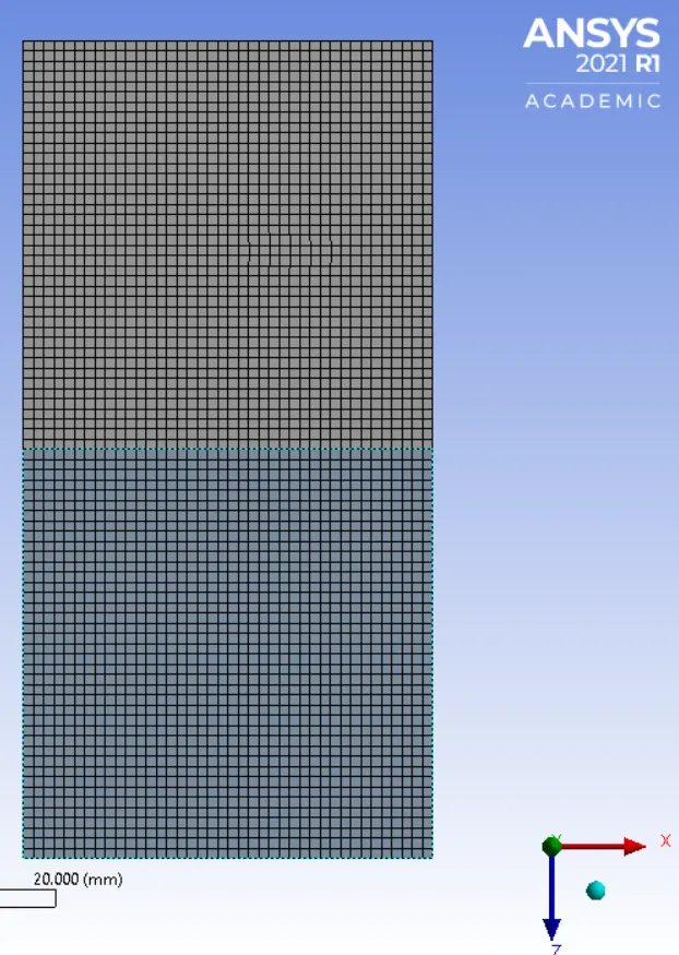
BASELINE MESH(0.5mm)
The baseline mesh is generated in order to observe the effects of RT instability on the computational domain.
1. Element Order: Linear
2. Element Size: 0.5mm
3. Number of Nodes : 3321
4. Number of Elements: 3200
Simulation Setup
1. Solver: Transient
2. Type : Pressure Based
3. Gravitational Acceleration:
- X: 0
- Y: - 9.81
4. Viscous Model: Laminar
5. Multiphase Model:
- Model: Volume of Fluid
- Number of Eulerian Phases: 2
- Formulation: Implicit
- Interference Modeling: Sharp
6. Material: Water & Air
7. Phases:
- Primary: Air
- Secondary: Water
8. Solution Method Scheme: SIMPLE
9. Solution Initialization:
- Method: Standard
Simulation Output
1. Residual:
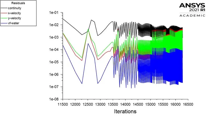
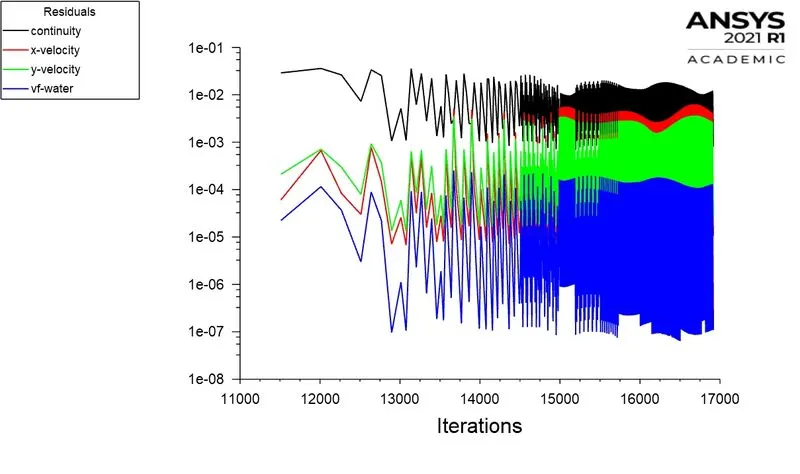
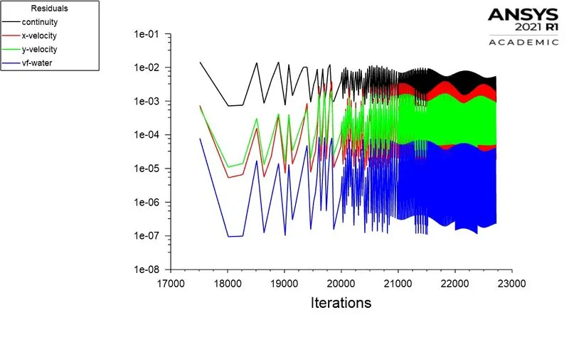
The residuals have an initial low order, before it begins to oscillate due to the Rayleigh Taylor instability. We can see that in the end stages of simulation, the residuals begin to oscillate periodically. Thus, we can assume that the solutions has coverged.
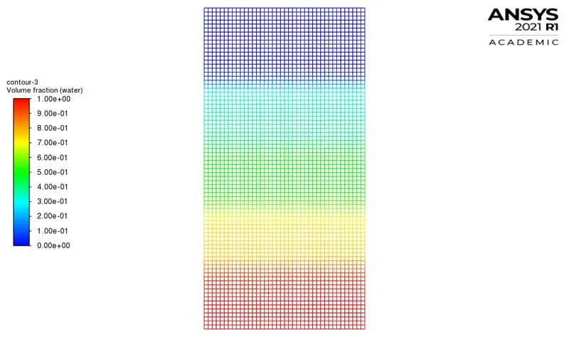
2. Contour of Volume Fraction( Water):
CASE-2
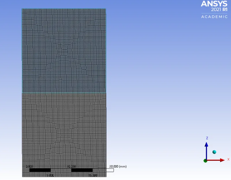
REFINED MESH (0.3mm)
The baseline mesh is generated in order to observe the effects of RT instability on the computational domain.
1. Element Order: Linear
2. Element Size: 0.3 mm
3. Number of Nodes : 9180
4. Number of Elements: 8978
Simulation Setup
The simulation setup is exactly the same as that for the baseline mesh. The simulation output will change due to the change in the mesh size.
Simulation Output
1. Residuals
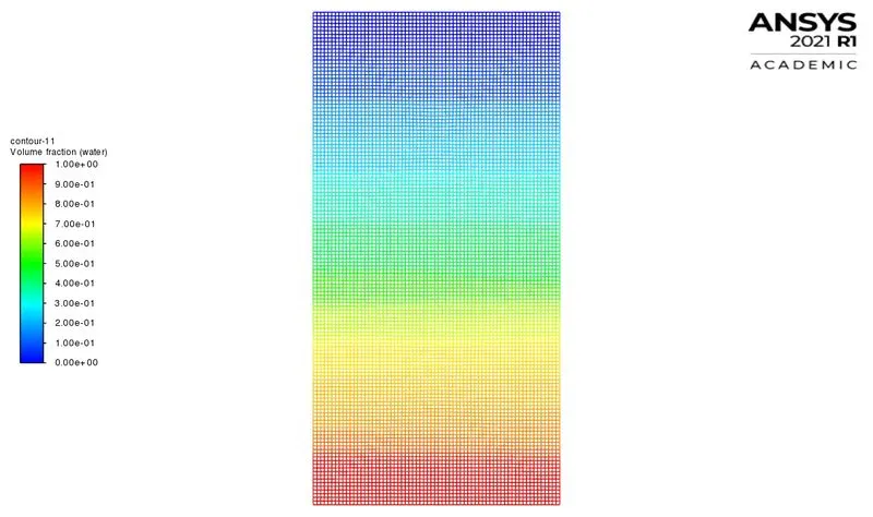
2. Contour of Volume Fraction( Water):
CASE-3
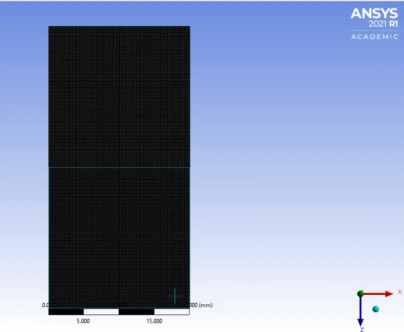
Refined Mesh( 0.15 mm)
The baseline mesh is generated in order to observe the effects of RT instability on the computational domain.
1. Element Order: Linear
2. Element Size: 0.15 mm
3. Number of Nodes : 35778
4. Number of Elements: 35378
Simulation Output
1. Residual
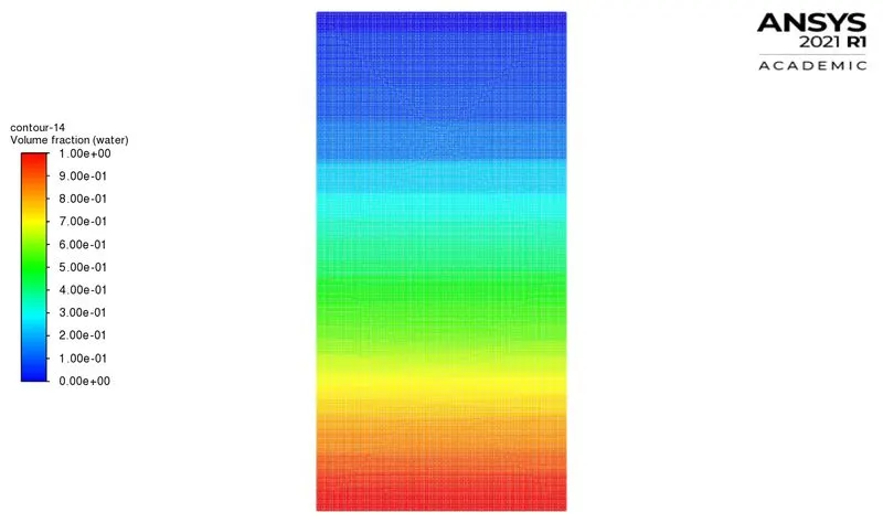
2. Contour of Volume Fraction( Water):
CASE-4
CUSTOM FLUID with ( 0.15 mm) refined mesh
The baseline mesh is generated in order to observe the effects of RT instability on the computational domain.
1. Element Order: Linear
2. Element Size: 0.15 mm
3. Number of Nodes : 35778
4. Number of Elements: 35378
Simulation Setup
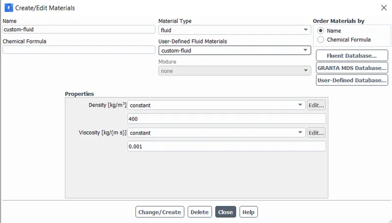
The simulation setup is exactly the same as that for the baseline mesh, except the custom fluid properties.The simulation output will change due to the change in the mesh size.
Simulation Output
1. Residual
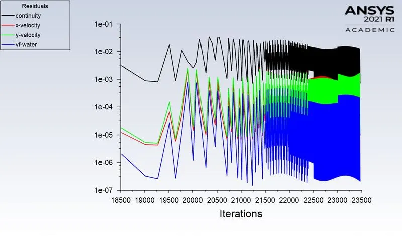
2. Contour of Volume Fraction( Water):
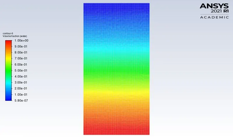
OBSERVATION:
We can observe that the final contour is much more detailed and accurate. This result can be considered to be highly accurate.
However, the time required to perform this simulation is also much higher than the previous meshes. Hence, only if an extremenly high accuracy is required from the solution, such a high degree of mesh refinement is suggested.
Atwood Number:
The Atwood number (A) is a dimensionless number in fluid dynamics used in the study of hydrodynamic instability in density stratified flows. It is a dimensionless density ratio defined as

where
- ρ1= density of heavier fluid
- ρ2= density of lighter fluid
Atwood number is an important parameter in the study of Rayleigh–Taylor instability and Richtmyer–Meshkov instability. In Rayleigh–Taylor instability, the penetration distance of heavy fluid bubbles into the light fluid is a function of acceleration time scale,Agt^2 where g is the gravitational acceleration and t is the time.
ATWOOD NUMBER CALCULATION:
A=(ρ1−ρ2)/(ρ1+ρ2)
For Air - Water RT instability
ρ1=9982.kg/m3
ρ2=1.225kg/m3
A=(998.2−1.225)/(998.2+1.225)
A=0.998
For Water - User Defined Material RT instability
ρ1=998.2kg/m3
ρ2=400kg/m3
A = (998.2−400)/(998.2+400)
A =0.428
The variation in Atwood number in the above 2 cases affects the behavior of the instability.
For Atwood number close to 0, RT instability flows take the form of symmetric fingers of fluid.
when Atwood number close to 1, the much lighter fluid below the heavier fluid takes the form of larger bubbles like plumes.
Therefore, from the value of Atwood number it is seen from the simulations that air forms larger bubbles when water is poured down the air pushes through and forms large bubbles. Therefore, the results can be validated by obtaining the value of Atwood number.
STEADY STATE VS TRANSIENT STATE:
The difference between the steady and Transient state is that you can't see the small-time variations of instability. The steady-state simulation is prefered, if we are concerend more about the final state results at the equilibrium state. In Rt -Instability CFD models, we are more concerened to learn about the transition of the irregularities that starts developing when we pour high dense fluid upon low dense fluid under gravity effect ,so by using transient solver along with refined mesh of the model, we can compute the smooth transition of irregualrities that takes place at the interface of the fluids. The final state results for both the steady-state and transient state will be the same.
In this problem we are observing the instabilities when it is occouring so we are not conserened about the final answer because steady stae is more into capturing the final results but by transient state we can see the behaviour of the solution and every instace such that capturing bubbles. vortex and shockwaves. So this is reason why transient is more suitable than steady-state model.
Google drive links:
https://drive.google.com/file/d/1XrAeJmEtE4t1rN6EY_KEv3o4qIC1myLW/view?usp=sharing
https://drive.google.com/file/d/1fm1juk_57h6QPWkIbfkdunRDwWGeAGCV/view?usp=sharing
https://drive.google.com/file/d/1fpOwO-zOmcuR3fURvHfvrVtKZoXsew1t/view?usp=sharing
https://drive.google.com/file/d/1hdRRSymPZSjLV4gvLfgmrRiOk85zgfE1/view?usp=sharing
RESULTS:
1. Due to the simplicity of the computational domain, the quality of mesh is extermely high.
2. Increasing the mesh size results in a more well - defined contour and also increases the accuracy of the solution.
3. The Atwood number, A = 0.998. Hence, the solution should give rise to bubbles - like plumes which can be clearly observed in the animation of the volume fraction of water, thus validating the results of the given problem.
CONCLUSION:
Atwood number forms a basis to compare and study research papers based on RT Instability. Thus we can use these papers to validate our results for better accuracy.