Week 3: Flow over a backward facing step
Aim:
To Simulate the flow over a backward facing step using converge.
Objective:
- To run the case for three different mesh grid
dx = dy = dz =2e-3m
dx = dy = dz =1.5e-3m
dx = dy = dz =1.0e-3m
- To show mesh for all three grid sizes.
- To Show pressure and velocity contours ,the plots of velocity, pressure, mass flow rate and total cell count for all the 3 base mesh sizes
- Explain Why separation takes place.0
Theory:
Flow separation:
Flow separation or boundary layer separation is the detachment of a boundary layer from a surface into awake. Separation occurs inflow that is slowing down, with pressure increasing, after passing the thickest part of a streamlined body. or It is a point at which the velocity gradient at the surface in a direction normal to the wall decreases to zero.
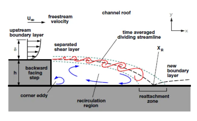
This separation happens due to the presence of either viscosity or pressure gradient or due to abrupt change in geometry. In most times it occurs due to the change in the geometry at sharp edges. From the below figure the flow was separated due to a change in the geometry. It shows the recirculation zone which happens due to flow separation. In this type of zones, zone eddies form i.e flow flows in a circular fashion. After that the recirculation zone is reattached and flow again happens over the surface.
Procedure:
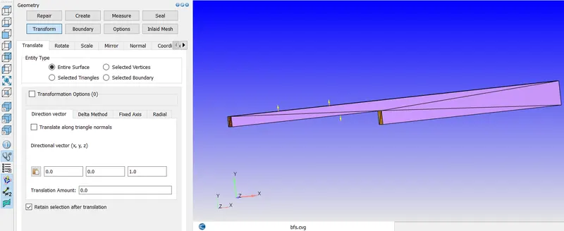
Load the geometry and assign the boundaries and check the direction of the normals. Actually, the normals should be pointed towards the flow of fluid or air in the channel. Enable the normals by clicking the normal toggle icon which is located on the bottom side in the left panel. If the normals are pointed reverse then select any triangle on the face whose normal is pointed away from the flow and select transform in the geometry toolbox > normal > click on propagate change from single triangle and press apply.
Material
Air (Predefined mixture) is used as the working fluid for performing gas simulation. Accordingly, the following global properties are utilized:
Turbulent Prandtl number: 0.9
Turbulent Schmidt number: 0.78
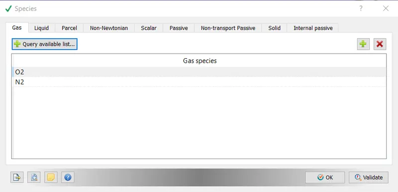
Species:
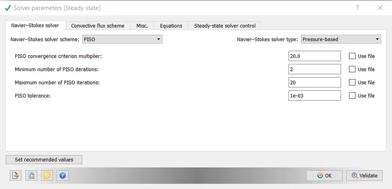
Run Parameters: Select steady-state solver in the solver and under Misc. uncheck the use shared memory and check the steady-state monitor and click on ok.
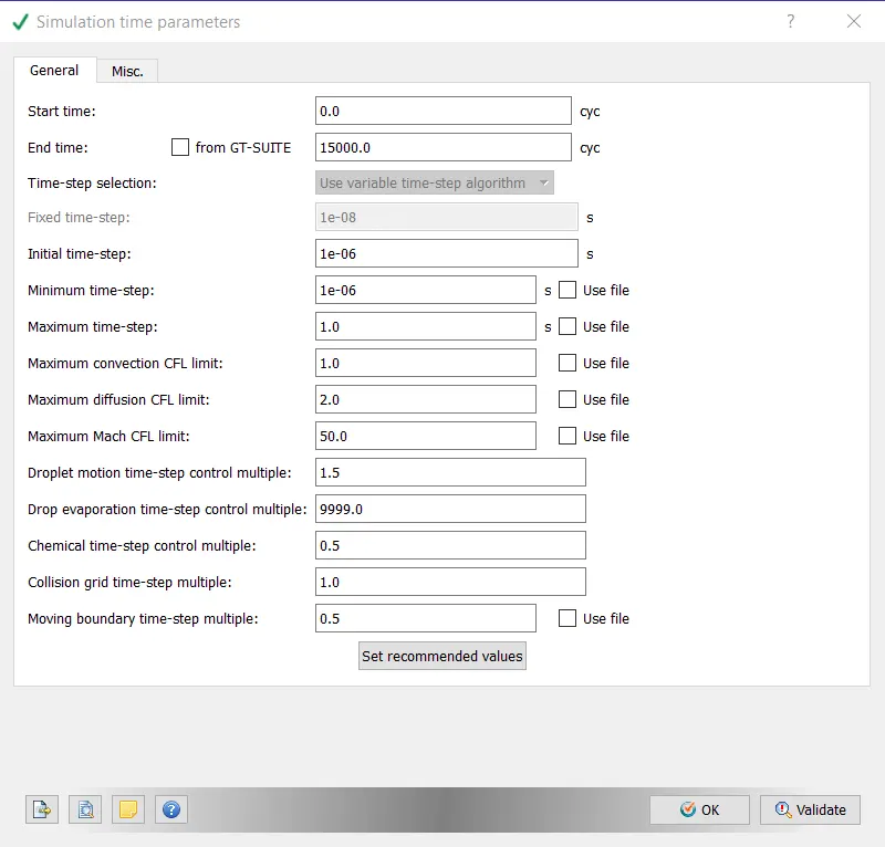
Simulation Time parameters:
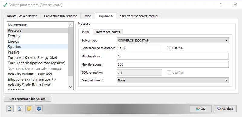
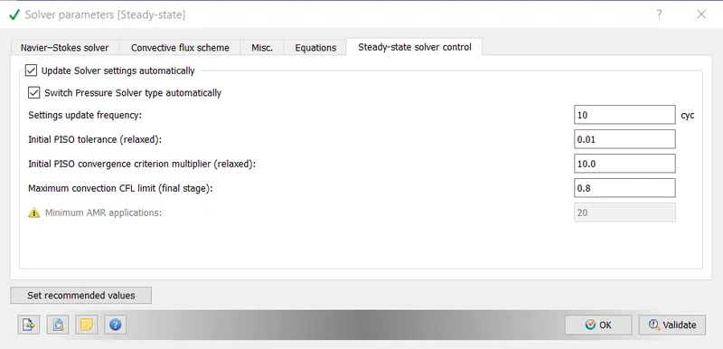
Solver parameters:
Regions and Initialization:
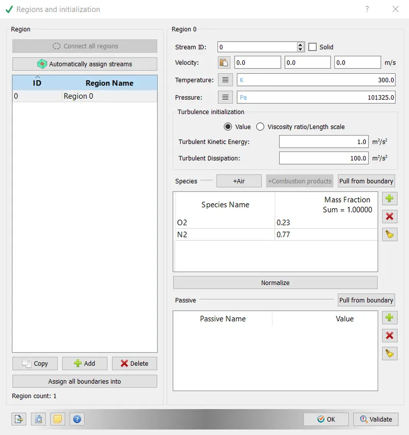
Initial conditions
The following settings are applied as the initial conditions:
Velocity: X component=0; Y component=0; Z component=0
Temperature: 300K
Pressure: 101325Pa
Species: Mass fractions: Oxygen: 0.23; Nitrogen: 0.77
Boundary conditions
The following boundary conditions are applied:
1. Inlet: INFLOW type boundary condition is applied with the following settings:
Total pressure: 110325Pa
Velocity: Zero normal gradient
Temperature: 300K
Species: Mass fractions: Oxygen: 0.23; Nitrogen: 0.77
2. Outlet: OUTFLOW type bundary condition is applied with the following settings:
Pressure: 101325Pa
Velocity: Zero normal gradient
Temperature backflow: 300K
Species backflow: Mass fractions: Oxygen:0.23; Nitrogen: 0.77
3. Wall: Wall type boundary condition is applied with the following settings:
Wall motion type: Stationary
Surface movement: FIXED
Velocity: Law of wall
Temperature: Law of wall; 300K
4. Front_2D: TWO_D type boundary condition is applied.
5. Back_2D: TWO_D type boundary condition is applied.
Grid control: Enable the fixed embedding check and click on ok. By using fixed embedding, we can get finer mesh around the top and bottom walls. This case study using 3 different mesh grid sizes. So, the different mesh grids are dx = dy = dz = 2e-3, 1.5e-3, and 1e-3.
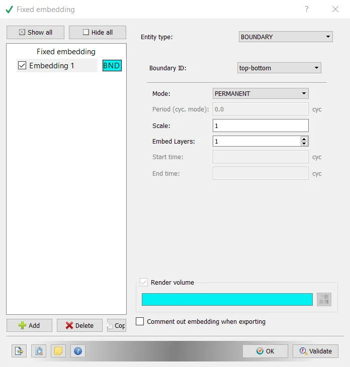
Now export all input files: Click on files > Export > Export input files > choose the path and select all files and press ok.
Run the simulation and post-convert the files: Copy and paste the mpiexec.exe file and converge.exe file to the folder in which the input files are exported to run the simulation in Cygwin. Copy the post_convert_30_msmpi_64.exe file and paste it into the output folder. Now open Cygwin and go to the output folder and type mpiexec.exe -n 4 post_convert_30_msmpi_64.exe > enter the case name(as case1) > select file type as Paraview VTK in-line binary format > type all for files and cell variables and click enter (or) we can convert those files in converge studio.
Post-processing the files:
To post-process the files lanch paraview and open the file location as case1 which is saved in output > case1 .. vtm (this is a group file which is formed during post-converting the files) > click on apply > create a slice along the z-axis.
Grid:
The following three meshes are used for simulations:
i. Mesh 1: Grid size: dx=dy=dz=2e-3m

ii. Mesh 2: Grid size: dx=dy=dz=1.5e-3m

iii. Mesh 3: Grid size: dx=dy=dz=1e-3m

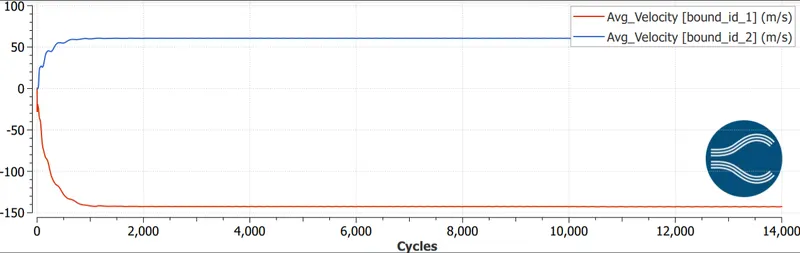
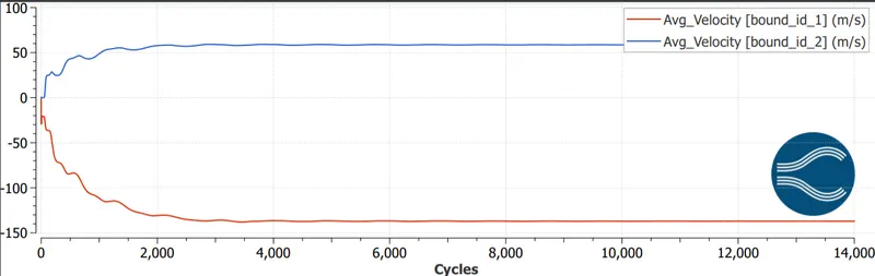
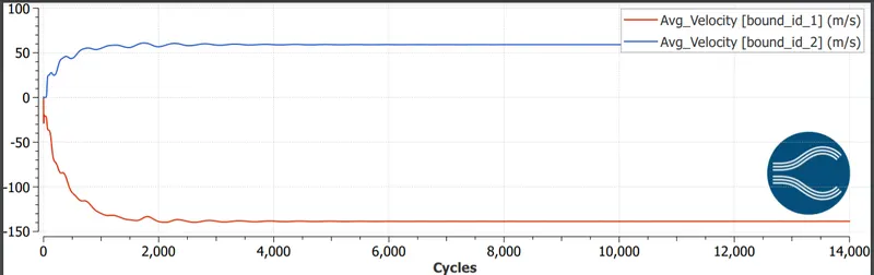
Average velocity vs simulation cycles:
Average velocity at inlet and outlet is plotted over simulation cycles, for all three meshes.
i. Mesh 1: Grid size: dx=dy=dz=2e-3m
ii. Mesh 2: Grid size: dx=dy=dz=1.5e-3m
iii. Mesh 3: Grid size: dx=dy=dz=1e-3m
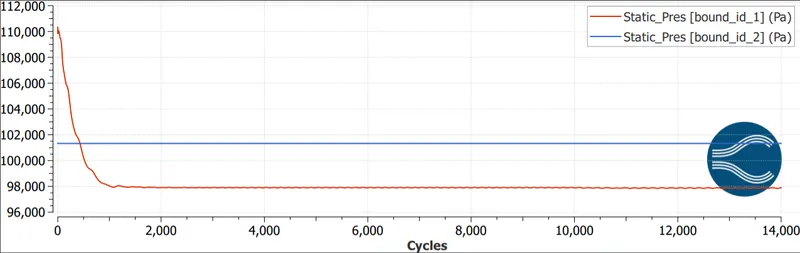
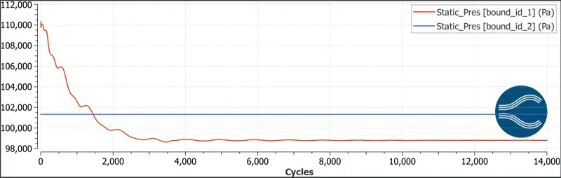
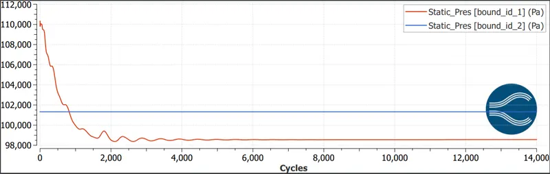
Static pressure vs simulation cycles:
Static pressure at inlet and outlet is plotted over simulation cycles, for all three meshes.
i. Mesh 1: Grid size: dx=dy=dz=2e-3m
ii. Mesh 2: Grid size: dx=dy=dz=1.5e-3m
iii. Mesh 3: Grid size: dx=dy=dz=1e-3m
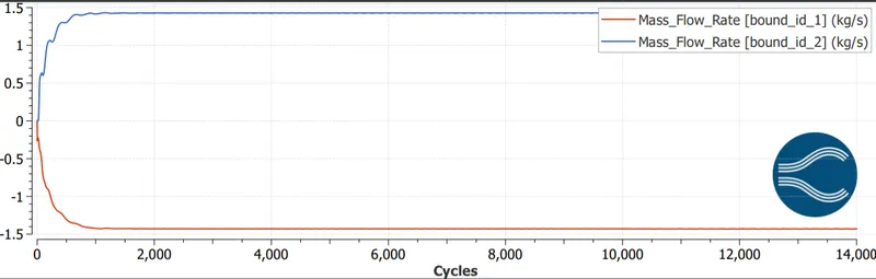
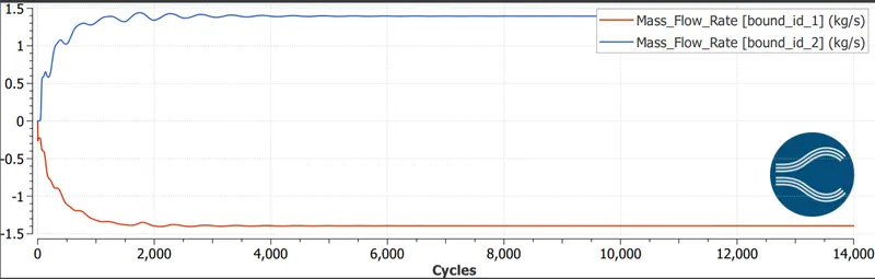
Mass flow rate vs simulation cycles:
Mass flow rate at inlet and outlet is plotted over simulation cycles, for all three meshes.
i. Mesh 1: Grid size: dx=dy=dz=2e-3m
ii. Mesh 2: Grid size: dx=dy=dz=1.5e-3m
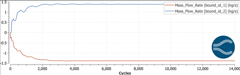
iii. Mesh 3: Grid size: dx=dy=dz=1e-3m
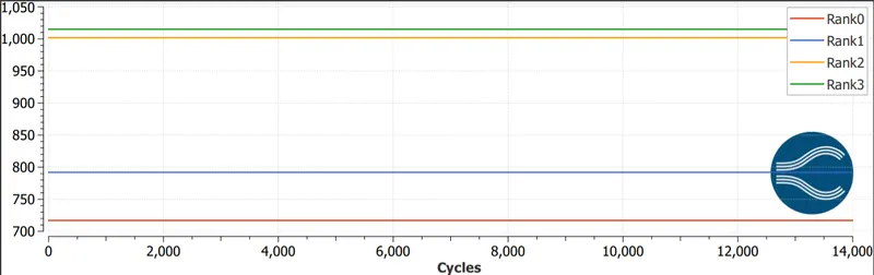
Cell count ranks:
Cell count ranks are plotted over simulation cycles, for all three meshes.
i. Mesh 1: Grid size: dx=dy=dz=2e-3m
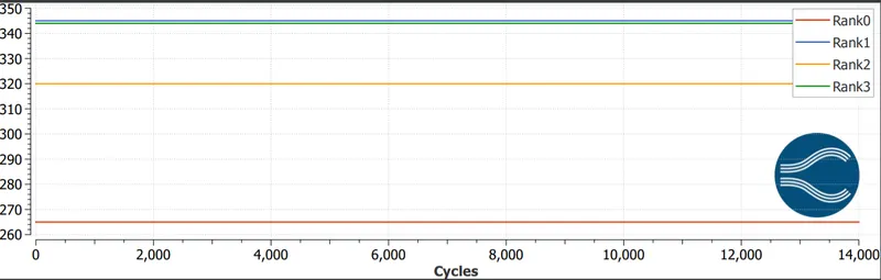
ii. Mesh 2: Grid size: dx=dy=dz=1.5e-3m
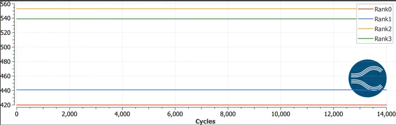
iii. Mesh 3: Grid size: dx=dy=dz=1e-3m
Velocity contours:
Velocity contours are plotted for all three meshes.
i. Mesh 1: Grid size: dx=dy=dz=2e-3m

ii. Mesh 2: Grid size: dx=dy=dz=1.5e-3m

iii. Mesh 3: Grid size: dx=dy=dz=1e-3m

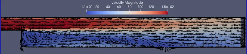
Velocity vectors:
Velocity vectors are plotted for all three meshes.
i. Mesh 1: Grid size: dx=dy=dz=2e-3m
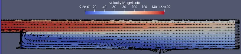
ii. Mesh 2: Grid size: dx=dy=dz=1.5e-3m
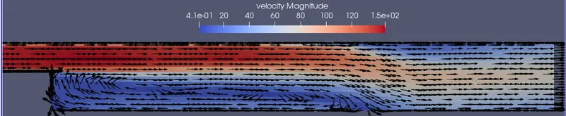
iii. Mesh 3: Grid size: dx=dy=dz=1e-3m
Pressure contours:
Pressure contours are plotted for all three meshes.
i. Mesh 1: Grid size: dx=dy=dz=2e-3m

ii. Mesh 2: Grid size: dx=dy=dz=1.5e-3m

iii. Mesh 3: Grid size: dx=dy=dz=1e-3m

Animation:
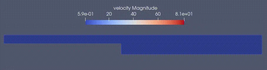
The animation attached below shows the development of velocity contours over simulation cycles, for Mesh 3.
Discussion:
i. The contour plots become more smooth and resolved with a decrease in grid size.
ii. The scales for contour plots indicate the following maxima for velocity magnitude: Mesh 1: 160m/s; Mesh 2: 150m/s; Mesh 3: 150m/s.
iii. The velocity vector plots for all three meshes indicate the presence of recirculation zones near the step.
iv. The plots for average velocity over simulation cycles indicate the following values of steady-state average velocity at the outlet: Mesh 1: 67.24m/s; Mesh 2: 65.42m/s; Mesh 3: 65.77m/s.
v. The plots for mass flow rate over simulation cycles show that for all three meshes a good mass conservation is achieved.
Conclusion:
- If the mesh size decreases, the results become more accurate and produce smooth plots due to increasing in the computation time.
- If the mesh size decreases, the converge decreases the time step to maintain the CFL number.