Week 7 - Simulation of a 1D Super-sonic nozzle flow simulation using Macormack Method

Nozzle:

A nozzle is a device designed to control the direction or characteristics of a fluid flow (to increase velocity) as its exists (or enters) an enclosed chamber or pipe. Nozzles are used to control the flow rate, speed,direction,mass,shape and pressure of the stream that emerges from them.

• For subsonic and sonic flows convergent nozzles are used.i.e, flow measuring and flow regulating devices.
• Convergent-Divergent nozzles are used for supersonic flows.

1D Supersonic nozzle:

The nozzle has convergent,throat and divergent section. In convergent section when Mach number is less than 1(M<1),this condition is called as subsonic flow through nozzle.Here velocity of fluid particle is less than sound speed.

Whereas, In convergent section when Mach number is greater tahn 1(M>1),this condition called as sonic flow through nozzle.Here velocity of fluid particle is more than sound speed.

In throat the Mach number is equal to 1(M=1), that means the sound speed is equal to fluid particle speed.

Mach number:

The mach number is a dimensionless quantity representing the ratio of flow velocity past a boundary to the local speed of the sound.

M=`u/c`

where

M is the mach number

u is the velocity of the moving aircraft

c is the speed of sound at the given altitude

Quasi-1D flow:

A quasi 1D flow is one in which all variables vary primarily along one direction,say x.A flow in a duct with slowly varying area A(x) is the case of intrest here.In practice this means that the slope of the duct walls is small. Also, the x-velocity component u dominates the y and z- components v and w.

Maccorkmack Method:

This method is employed to solve the governing equations of quasi 1D supersonic nozzle flow rather than the differencing schemes as we have studied earlier.Maccorkmack method is an explicit finite difference technique which is second order accurate in both time and space. In CFD, the Maccorkmack method is a widely used discretization equations. This method essentially usues a predictor and corrector step.

Predictor Step-

In this the spatial terms on the right-side of the equation are replaced by forward differences. The RHS of the eqn is known as all the variables are for time step 't'. Next, the value of the LHS is calculated by employing the time marching solution and for the time-step 't+dt' values of the variable at all grid points is obtained.

Corrector Step-

In this the spatial terms on the right-side of the equation are replaced by backward differences. The value of variables in RHS are taken which are obtained in the predicted step for time-step ' t+dt'.

Governing equations for Quasi 1D supersonic nozzle flow:

The continuity, momentum and energy equations for Quasi 1D steady isentropic flow is given by

Continuity Eqn: ρ₁V₁A₁=ρ₂V₂A₂

Momentum Eqn: ρ₁ A₁+ ρ₁ V²₁+∫pdv= ρ₂ A₂+ ρ₂ V²₂

Energy Eqn: h1+ V²₁/2= h2+ V²₂/2

Calculation of Time step-

In order for the solution to be stable,the concept of courant flow number was introduced in previous projects. For a linear hyperbolic eqn, the value of CFL<1 will gibe stable solution.

For this project,CFL=0.5 and value of time-step is calculated as follows

△t=c(△x/(V+a))

where , C is courant number,

V is the local flow velocity at a point

a is the local speed of sound

Value of dt at all grid ponits is calculated and the minimum of them is chosen for the simulation.

Boundary Conditions:

@ Inlet:

Velocity at the inlet is changing with time, while the density and temperature are constant with respect to time.

u1=2u2+u3

Velocity at inlet is calculated by the method of linear extrapolation. Values of velocity at node 2 and 3 are used for the same.

@ Outlet:

All the variables at the outlet are kept changing with respect to time and linear extrapolation is used to calculate the variables at the outlet.

u_N=2u_N-1+u_N-2

T_N=2T_N-1+T_N-2

ρ_N=2 ρ_N-1+ ρ_N-2

Initial conditions:

Area of the nozzle will remain constant throughout the time of simulation.

A=1+2.2(x-1.5)^2

The flow field variables vary with respect to time. At t=0, their values are given as

ρ1+0.3146x

T=1+0.2314x

u=(0.1+1.09x)*T^0.5

Conservative Form:

The governing eqn are expressed in a generic form which consists of the solution vector U, the flux vector F and the source term J.

∂U/∂t +(∂F/∂x)=J

The equations for Quasi 1D supersonic flow can be expressed in a similar generic form

U1=ρAF1=ρAu

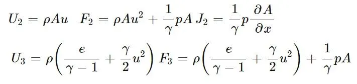
The equations which are solved using Maccormack method are

∂U₁/∂t = ∂F₁/∂x ∂U₂/∂t=-∂F₂/∂x+J₂

∂U₃/∂t=-∂F₃/∂x

Further, the flux vectors and source terms are expressed in terms of solution vectors.Also, to find the field variables, they are written in terms of solution vectors.

F₁=U₁

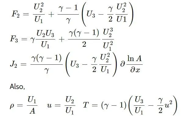
Calculation of time step is the same as that of the procedure followed for non-conservative form.

Boundary conditions:

@ Inlet:

U2 and U3 are changing with resoect to time whereas U1 is kept as constant.

U_2(i=1)=U_2(i=2)-U_2(i=3)

@ Oulet:

U1_(n)=2U_1(n-1)-U_1(n-2)

U2_(n)=2U_2(n-1)-U_2(n-2)

U_3(n)=2U_3(n-1)-U_3(n-2)

Initial conditions:

Area of the nozzle is constant throughout the runtime of simulation and its value is same as that taken for non-conservative from.

Initial velocity is given as

u=0.59/ρA

At t=0, values of density and temperature throughout the nozzle are given as folloes

rho'=1.0T'=1.0 ' for 0≤x'≤0.5

ρ'=1.0-0.366(x'-0.5) T'=1.0-0.167(x'-0.5) for

0.5≤x'≤1.5

ρ'=0.634-0.387(x'-1.5)

T'=0.833-0.3507(x'-1.5) for 1.5≤x'≤3.5

Matlab Code

Main code

clear all
close all
clc
%input variables

n=31;
L=3;
x=linspace(0,L,n);
%courant 
cf1=0.5;
%nodes @ throat
th=((n-1)/2)+2;
%time steps
nt=1400;

tic
%fun for non conservative form
[v_nc,rho_nc,T_nc,mass_nc,M_nc,p_nc,v_throat_nc,rho_throat_nc,T_throat_nc,mass_throat_nc,M_throat_nc,p_throat_nc]=non_conservative_approach(n,L,cf1,nt,th);
%calculating the simulation time
Non_conservative_simulation_time=toc;

tic
%fun for conservative form
[v_c,rho_c,T_c,mass_c,M_c,p_c,v_throat_c,rho_throat_c,T_throat_c,mass_throat_c,M_throat_c,p_throat_c]=conservative_approach(n,L,cf1,nt,th);
%calculating the simulation time
conservative_simulation_time=toc;

%analytical soln steady state
rho_an=0.634*ones(900,1400);
T_an=0.833*ones(900,1400);
p_an=0.528*ones(900,1400);
M_an=1*ones(900,1400);

figure(5)
a1=subplot(4,1,1);
plot(linspace(1,nt,nt),rho_throat_nc);
hold on
plot(linspace(1,nt,nt),rho_throat_c,'g');
hold on
plot(linspace(1,nt,nt),rho_an,'k');
hold on
grid on
ylabel('density')
legend('Non-conservative approach','conservative approach','Analytical approach')
title('variation in parameter at throat w.r to time step')

a2=subplot(4,1,2);
plot(linspace(1,nt,nt),T_throat_nc);
hold on
plot(linspace(1,nt,nt),T_throat_c);
hold on
plot(linspace(1,nt,nt),T_an);
hold on
grid on
ylabel('Temperature')
legend('Non-conservative approach','conservative approach','Analytical approach')
title('variation in parameter at throat w.r to time step')

a3=subplot(4,1,3);
plot(linspace(1,nt,nt),p_throat_nc);
hold on
plot(linspace(1,nt,nt),p_throat_c);
hold on
plot(linspace(1,nt,nt),p_an);
hold on
grid on
ylabel('pressure')
legend('Non-conservative approach','conservative approach','Analytical approach')
title('variation in parameter at throat w.r to time step')

a4=subplot(4,1,4);
plot(linspace(1,nt,nt),M_throat_nc);
hold on
plot(linspace(1,nt,nt),M_throat_c);
hold on
plot(linspace(1,nt,nt),M_an);
hold on
grid on
ylabel('Mach muber')
legend('Non-conservative approach','conservative approach','Analytical approach')
title('variation in parameter at throat w.r to time step')

figure(6)
b1=subplot(4,1,1);
plot(x,rho_nc)
hold on
plot(x,rho_nc,'*')
hold on
grid on
ylabel('density')
legend('Non-conservative approach','conservative approach','Analytical approach')
title('variation in properties along X')

b2=subplot(4,1,2);
plot(x,T_nc)
hold on
plot(x,T_nc,'*')
hold on
grid on
ylabel('Temperature')
legend('Non-conservative approach','conservative approach')
title('variation in properties along X')

b3=subplot(4,1,3);
plot(x,p_nc)
hold on
plot(x,p_nc,'*')
hold on
grid on
ylabel('pressure')
legend('Non-conservative approach','conservative approach')
title('variation in properties along X')

b4=subplot(4,1,4);
plot(x,M_nc)
hold on
plot(x,M_nc,'*')
hold on
grid on
ylabel('Mach number')
legend('Non-conservative approach','conservative approach')
title('variation in properties along X')

%mass flow rate comparision b/w two froms
figure(7)
plot(x,mass_nc)
hold on
plot(x,mass_c,'g')
hold on
plot(x,linspace(0.579,0.579,n),'k')
hold on
ylabel('Non-dimensionless mass flow rate')
legend('Non-conservative approach','conservative approach','Analytical approach')
title('Non-dimensionless mass flow rate comparision')
axis([0 3 0.55 .6])
grid on

y=[rho_nc(th) rho_c(th) 0.634; T_nc(th) T_c(th) 0.833; p_nc(th) p_c(th) 0.528; M_nc(th) M_c(th) 1];
x_axis= categorical({'1.density','2.Temperature','3.pressure','4.Mach number'});

figure(10)
labels={'Non-conservative approach','conservative approach','Analytical approach'};
b=bar(x_axis,y,'group');
legend(labels,'location','northoutside','orientation','vertical')
a=(1:size(y,1)).';
x_ax=[a-0.25 a a+0.25];
for k=1:size(y,1)
    for m=1:size(y,2)
        text(x_ax(k,m),y(k,m),num2str(y(k,m),'%0.2f'),'Horizontalalignment','center','verticalalignment','bottom')
    end
end

For non consecutive approach

function[v,rho,T,mass,M,p,v_throat,rho_throat,T_throat,mass_throat,M_throat,p_throat]=non_conservative_approach(n,L,cf1,nt,th)
%inputs
n=31;
L=3;
x=linspace(0,3,n);
dx=x(2)-x(1);

%conditions
rho=1-0.3146*x;
T=1-0.2314*x;
v=(0.1+1.09*x).*T.^0.5;
a=1+2.2*(x-1.5).^2;
th=find(a==1);
gamma=1.4;

%time steps
cf1=0.5;
dt=min(cf1.*(dx./((sqrt(T))+v)));
%number of iterations
nt=1400;
%rho_initial=rho;
%T_initial=T;
%v_initial=v;
for k=1:nt
    %copy of the variables
    rho_old=rho;
    T_old=T;
    v_old=v;
    
%predictor step
  for j=2:n-1
    dv_dx=(v(j+1)-v(j))/dx;
    drho_dx=(rho(j+1)-rho(j))/dx;
    dTdx=(T(j+1)-T(j))/dx;
    da_dx=(log(a(j+1))-log(a(j)))/dx;
    %continuity
    drhodt_p(j)=-rho(j)*dv_dx-rho(j)*v(j)*da_dx-v(j)*drho_dx;
    %momentum
    dvdt_p(j)=-v(j)*dv_dx-(1/gamma)*(dTdx+(T(j)/rho(j))*drho_dx);
    %energy
    dTdt_p(j)=-v(j)*dTdx-(gamma-1)*T(j)*(dv_dx+v(j)*da_dx);
    %solution updates
    v(j)=v(j)+dvdt_p(j)*dt;
    T(j)=T(j)+dTdt_p(j)*dt;
    rho(j)=rho(j)+drhodt_p(j)*dt;
  end
%corrector method
  for j=2:n-1
    dv_dx=(v(j)-v(j-1))/dx;
    drho_dx=(rho(j)-rho(j-1))/dx;
    dTdx=(T(j)-T(j-1))/dx;
    da_dx=(log(a(j))-log(a(j-1)))/dx;
    %continuity
    drhodt_c(j)=-rho(j)*dv_dx-rho(j)*v(j)*da_dx-v(j)*drho_dx;
    %momentum
    dvdt_c(j)=-v(j)*dv_dx-(gamma^-1)*(dTdx+(T(j)/rho(j))*drho_dx);
    %energy
    dTdt_c(j)=-v(j)*dTdx-(gamma-1)*T(j)*(dv_dx+v(j)*da_dx);
  end
%average
dvdt_avg=0.5*(dvdt_c+dvdt_p);
drhodt_avg=0.5*(drhodt_c+drhodt_p);
dTdt_avg=0.5*(dTdt_p+dTdt_c);
%soln update
  for i=2:n-1
    v(i)=v_old(i)+dvdt_avg(i)*dt;
    T(i)=T_old(i)+dTdt_avg(i)*dt;
    rho(i)=rho_old(i)+drhodt_avg(i)*dt;
  end

%inlet condition by interpolation
v(1)=2*v(2)-v(3);
%outlet condition by interpolation
v(n)=2*v(n-1)-v(n-2);
T(n)=2*T(n-1)-T(n-2);
rho(n)=2*rho(n-1)-rho(n-2);

%properties
mass=rho.*a.*v;
M=v./((T).^0.5);
p=rho.*T;
%throat values
rho_throat(k)=rho(th);
v_throat(k)=v(th);
T_throat(k)=T(th);
M_throat(k)=M(th);
p_throat(k)=p(th);
mass_throat(k)=mass(th);

%residues at throat.
v_res(k)=dvdt_avg(th);
rho_res(k)=drhodt_avg(th);
T_res(k)=dTdt_avg(th);

%plots

figure(1)
 if k==50
    plot(x,mass,'b','linewidth',1.5)
    hold on
elseif k==100
    plot(x,mass,'r','linewidth',1.5)
    hold on
elseif k==150
    plot(x,mass,'c','linewidth',1.5)
    hold on
elseif k==200
    plot(x,mass,'g','linewidth',1.5)
    hold on
elseif k==550
    plot(x,mass,'y','linewidth',1.5)
    hold on
elseif k==700
    plot(x,mass,'k','linewidth',1.5)
    hold on
elseif k==1400
    plot(x,mass,'m','linewidth',1.5)
    grid on
    ylabel('mass flow rate')
    xlabel('nozzle length(x)')
    title('mass flow rate at different time steps non conservative approach')
    legend('50 time steps','100 time steps','150 time steps','200 time steps','550 time steps','700 time steps','1400 time steps')
 end
end

figure(3)
plot(linspace(1,nt,nt),v_res);
hold on
plot(linspace(1,nt,nt),rho_res,'g');
hold on
plot(linspace(1,nt,nt),T_res,'k');
grid on
ylabel('residues')
xlabel('timestep')
legend('vplot','rhoplot','Tplot')
title('residual plot')
end

For consecutive approach

function[v,rho,T,mass,M,p,v_throat,rho_throat,T_throat,mass_throat,M_throat,p_throat]=conservative_approach(n,L,cf1,nt,th)
%geo
L=3;
n=31;
x=linspace(0,L,n);
dx=x(2)-x(1);

%initial conditions
a=1+2.2*(x-1.5).^2;
th=find(a==1); %throat node
rho_initial=ones(1,n);
T_initial=ones(1,n);

 for i=1:n
    if (x(i)<=0.5)
        rho_initial(i)=1;
        T_initial(i)=1;
    elseif (x(i)>=0.5 && x(i)<=1.5)
        rho_initial(i)=1-0.366*(x(i)-0.5);
        T_initial(i)=1-0.167*(x(i)-0.5);
    elseif (x(i)>=1.5 && x(i)<=3)
        rho_initial(i)=0.634-0.3879*(x(i)-1.5);
        T_initial(i)=0.833-0.3507*(x(i)-1.5);
    end
 end

v=0.59./(rho_initial.*a);
gamma=1.4;

%solution term
p=rho_initial.*T_initial;
u1=rho_initial.*a;
u2=rho_initial.*a.*v;
u3=u1.*((T_initial/(gamma-1))+(0.5*gamma*v.^2));

%time step cal
cf1=0.5;
dt=min(cf1.*(dx./((sqrt(T_initial))+v)));
%No.of iterations
nt=1400;

rho=rho_initial;
T=T_initial;

%time loop

 for k=1:nt
    
    %copy of solution terms
    u1old=u1;
    u2old=u2;
    u3old=u3;
    
    %flux terms
    
    f1=u2;
    term=(((gamma-1)/gamma)*(u3-((gamma/2)*((u2.^2)./u1))));
    f2=((u2.^2)./u1)+term;
    f3=((gamma*u2.*u3)./u1)-(gamma*(gamma-1)*(u2.^3))./(2*u1.^2);
    
    %predcitor step
      for i=2:n-1
          df1dx(i)=(f1(i+1)-f1(i))/dx;
          df2dx(i)=(f2(i+1)-f2(i))/dx;
          df3dx(i)=(f3(i+1)-f3(i))/dx;
          dlogadx(i)=(log(a(i+1))-log(a(i)))/dx;
        
          dadx(i)=(a(i+1)-a(i))/dx;
          j2(i)=(1/gamma)*rho(i)*T(i)*dadx(i);
        
        %continuity eqn
          du1dt_p(i)=-df1dx(i);
        %momentum eqn
          du2dt_p(i)=-df2dx(i)+j2(i);
        %energy eqn
          du3dt_p(i)=-df3dx(i);
        
        %soln update
          u1(i)=u1(i)+du1dt_p(i)*dt;
          u2(i)=u2(i)+du2dt_p(i)*dt;
          u3(i)=u3(i)+du3dt_p(i)*dt;
      end
    
    %primitive variables
    rho=u1./a;
    v=u2./u1;
    T=(gamma-1)*((u3./u1)-((gamma*v.^2)/2));

    %flux terms befor corrector step
    f1=u2;
    term=(((gamma-1)/gamma)*(u3-(gamma*u2.^2)./(2*u1)));
    f2=((u2.^2)./u1)+term;
    f3=((gamma*u2.*u3)./u1)-((gamma*(gamma-1)/2)*((u2.^3)./(u1.^2)));
        
    %corrector method
      for i=2:n-1
          df1dx(i)=(f1(i)-f1(i-1))/dx;
          df2dx(i)=(f2(i)-f2(i-1))/dx;
          df3dx(i)=(f3(i)-f3(i-1))/dx;
          dlogadx(i)=(log(a(i+1))-log(a(i)))/dx;
          dadx(i)=(a(i)-a(i-1))/dx;
          j2(i)=(1/gamma)*rho(i)*T(i)*dadx(i);
        
        %continuity eqn
          du1dt_c(i)=-df1dx(i);
        %momentum eqn
          du2dt_c(i)=-df2dx(i)+j2(i);
        %energy eqn
          du3dt_c(i)=-df3dx(i);
      end
    
    %average derivative
    du1dt=0.5*(du1dt_c+du1dt_p);
    du2dt=0.5*(du2dt_c+du2dt_p);    
    du3dt=0.5*(du3dt_c+du3dt_p);    
    
    %final soln update
       for j=2:n-1
        u1(j)=u1old(j)+du1dt(j)*dt;
        u2(j)=u2old(j)+du2dt(j)*dt;
        u3(j)=u3old(j)+du3dt(j)*dt;
       end
        %inlet condition
        u1(1)=rho(1)*a(1);
        u2(1)=2*u2(2)-u2(3);
        v(1)=u2(1)/u1(1);
        u3(1)=u1(1)*((T(1)/(gamma-1))+(0.5*gamma*v(1)^2));
        
        %outlet boundary
        u1(n)=2*u1(n-1)-u1(n-2);
        u2(n)=2*u2(n-1)-u2(n-2);
        u3(n)=2*u3(n-1)-u3(n-2);
        
        %primitive terns
        rho=u1./a;
        v=u2./u1;
        T=(gamma-1)*((u3./u1)-(gamma/2)*(v.^2));
        
        %properties
        mass=rho.*a.*v;
        M=v./((T).^0.5);
        p=rho.*T;
        
        %throat values
        rho_throat(k)=rho(th);
        v_throat(k)=v(th);
        T_throat(k)=T(th);
        M_throat(k)=M(th);
        p_throat(k)=p(th);
        mass_throat(k)=mass(th);
        
        %residues at throat
        u1_res(k)=du1dt(th);
        u2_res(k)=du2dt(th);
        u3_res(k)=du3dt(th);
        
  %plot
  
  figure(2)
  if k==50
    plot(x,mass,'b','linewidth',1.5)
    hold on
elseif k==100
    plot(x,mass,'r','linewidth',1.5)
    hold on
elseif k==150
    plot(x,mass,'c','linewidth',1.5)
    hold on
elseif k==200
    plot(x,mass,'g','linewidth',1.5)
    hold on
elseif k==550
    plot(x,mass,'y','linewidth',1.5)
    hold on
elseif k==700
    plot(x,mass,'k','linewidth',1.5)
    hold on
elseif k==1400
    plot(x,mass,'m','linewidth',1.5)
    grid on
    ylabel('mass flow rate')
    xlabel('nozzle length(x)')
    title('mass flow rate at different time steps conservative approach')
    legend('50 time steps','100 time steps','150 time steps','200 time steps','550 time steps','700 time steps','1400 time steps')
  end
 end
        
figure(4)
plot(linspace(1,nt,nt),u1_res)
hold on
plot(linspace(1,nt,nt),u2_res,'g')
hold on
plot(linspace(1,nt,nt),u3_res,'k')
grid on
ylabel('residues')
xlabel('timestep')
legend('u1plot','u2plot','u3plot')
title('residual plot')
end

Graphs and Explanation:

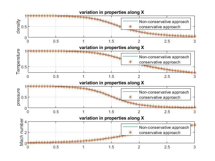
1.Variation of low properties along the nozzle length

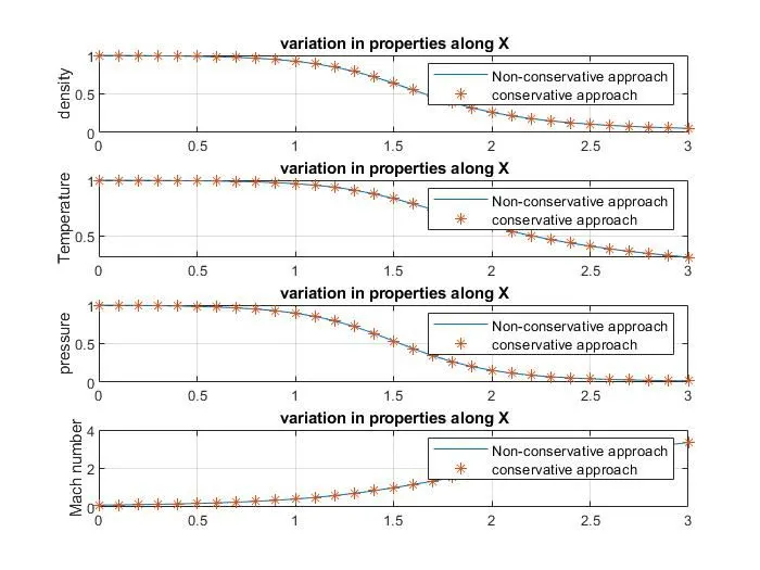
we can observe that both conservative and non conservative approach are in close point in an nozzle.

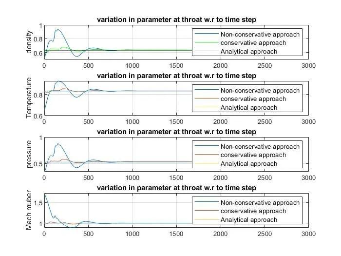
2. Variation of low properties with time step at throat

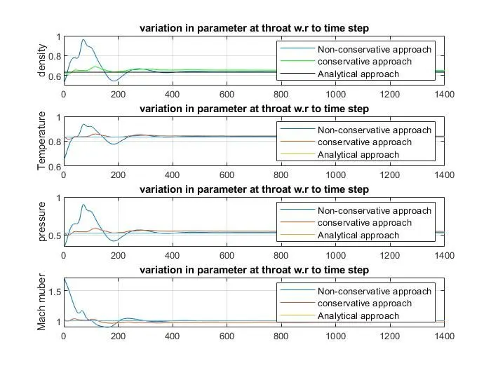
• From the graph we can see that both the conservative and non-conservative tends to steady state after 600th time step.
• Non-Conservative solutions is in more close agreement with analytical solution than the conservative solution
• The plot that the stability is achieved by the non-conservative form earlier than the conervative form but the amplitude of the initial variations is also higher in the non-conservative form. Also the convergence criterua has been kept equal for both the cases.

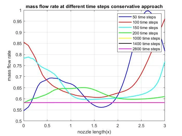
3.Mass flow rate variation along X at different time steps-Conservative approach

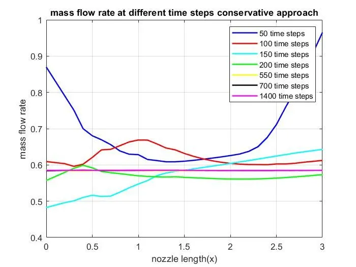
It can be seen that the curve for 550, 700 and 1400 time steps are close and lie in the same band. The fluctuations are less as we assumed to have constants mass flow rate initially.

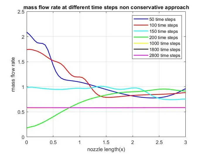
4.Mass flow rate variation along X at different time steps non-Conservative approach

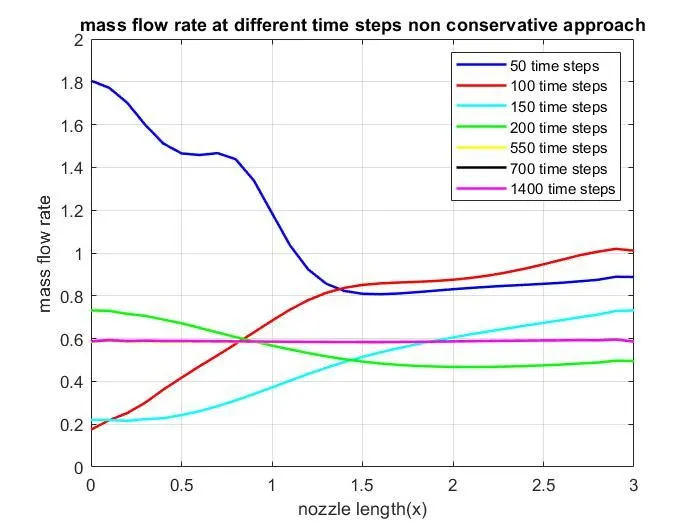
Even here we can see that the curve for 550, 700 and 1400 time steps lie in the same band are close. The fluctuations are high as the mass flow rate is derived from other parameter.

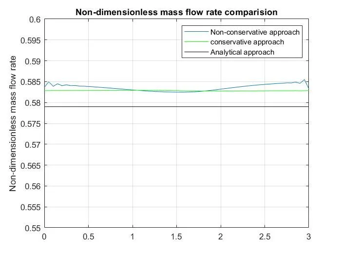
5.Comparision of mass flow rate

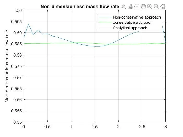
Conservative curve is smooth and lies close to the analytical value since mass flow rate is directly calculated and the assumption in the begining is to have to a constant mass flow rate.

Non-Conservative approaches close to the analytical value only at the throat.

The profile od the conservative form is much closer to the exact solution and on the other hand the variation in the mass flow rate of the non-conservative from is larger and also far from the eaxct ananlytical solution.

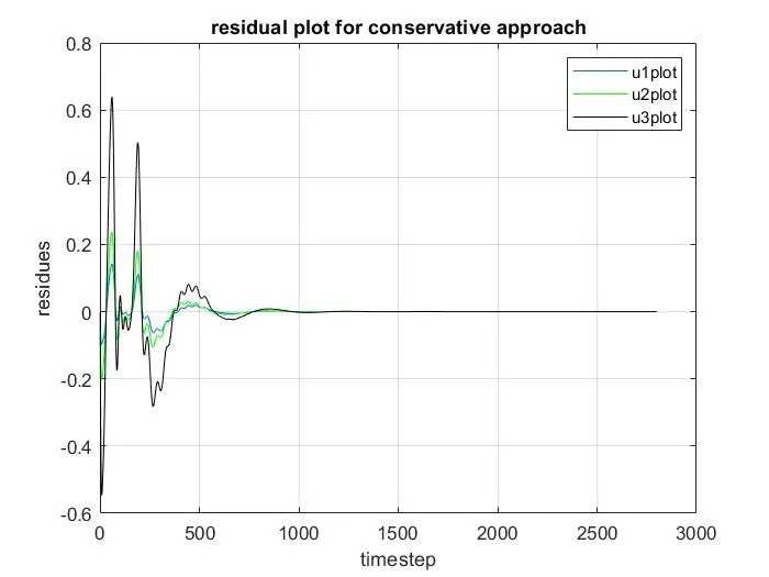
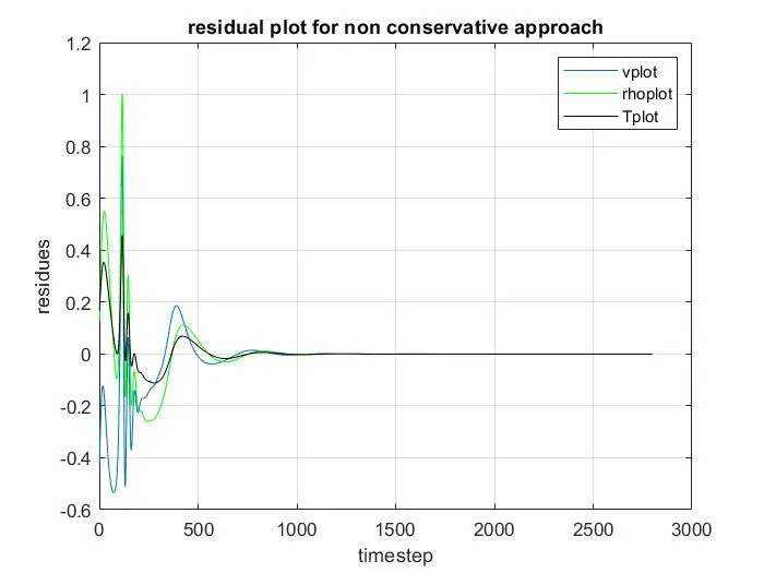
6.Residual graphs

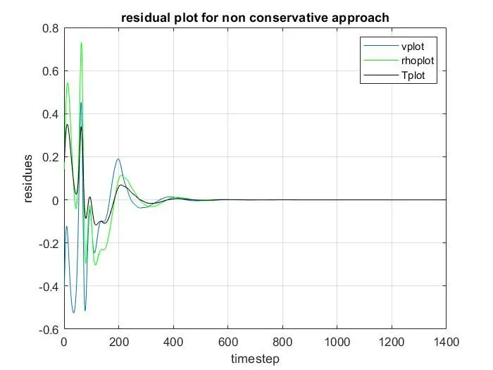
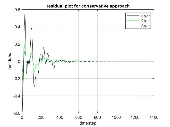
All the residuals from the graph for conservative and non conservative is converging at time step 800 and 600 respectively.

Grid Dependency:

The solution is said to be grid independent if the solution has no effect even if the number of grid points are increased once the stable solution is obtained.

Now, let us double the number of grid points to 61 and accordingly the dt should be changed.This can be obtained from the time step calculation from courant number for each grid.

1.Variation of flow properties along the nozzle length

2.Variation of flow properties with time step at throat

3.Mass flow rate variation along the X at different time steps conservative approach

4.Mass flow rate variation along the X at different time steps non-conservative approach

5.Comparision in mass flow rate

6.Residual graphs

SUMMARY:

For n=31 grid points

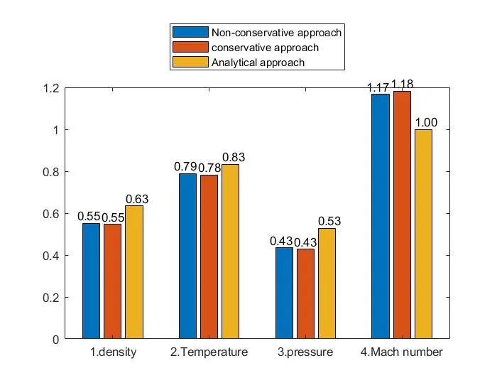
For n=61 grid points

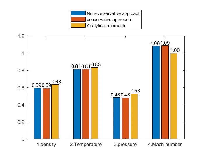
Comparing the plots of the grid size n=31 and n=61 it can be conclude that the solution is grid independent and solving conservative approach requires more computational effort and time than non conservative approach.

CONCLUSION:

	Conservative	Non-Conservtive
n=31	1000	600
n=61	1300	1000

The flow through the quasi 1D nozzle is subsonic at the convergenct section, transonic at the throat section and supersonic at the divergent section.

The number of iterations and the time for convergence is lesser in non-conservative form. Therefore it can be concluded that Non-Conservative form is faster than Conservative form but conservative form is more accurate.