Week 4 - Genetic Algorithm

AIM:

1. To optimize the stalagmite function using the GENETIC ALGORITHM approach.

2. To also find out the global maxima of the above function.

INTRODUCTION:

1. The stalagmite function is a mathematical function and it's function defenition is given below:

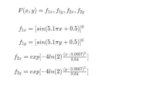
2. We are asked to optimize this function. Optimization is done by the GENETIC ALGORITHM approach. Optimization is nothing but the selection of the best element among a set of given alternatives.

3. The GENETIC ALGORITHM approach uses the charles darwin theory of evolution, where only the fittest individuals are selected for the generation of future offsprings. It is done in three steps:

a). Selection : We first define a population limit and it's size and we select some candidates based on their fitness value.

b). Crossover : We bring our selected candidates to the mating pool and we let them mate. The offspring is generated and it carries genes from both parents.

c). Mutation : After the offsprings are created, their genes are subjected to variation. This is called mutation, and this prevents the solution from falling. (going into a local minima)

4. We are also asked to find the global maxima of this function. In mathematical functions, there are local maxima and minima, as well as global maxima and minima. Global maxima and minima are the maximum and minimum values of the function's entire range. Local maxima and minima are the maximum and minimum values of the function in a given specific range.

Let us look at the MATLAB program and its code explanation.

PROCEDURE:

1. The program for the genetic algorithm is given below:

clear all
close all
clc

% Search space
x = linspace(0,0.6,150);
y = linspace(0,0.6,150);
num_case = 50;

% Generating a 2-D mesh
[xx yy] = meshgrid(x,y);

% Stalagmite function
for i = 1:length(xx)
    for j = 1:length(yy)
        input_vector(1) = xx(i,j);
        input_vector(2) = yy(i,j);
        f(i,j) = stalagmite(input_vector);
    end
end

% Case1
tic

for i = 1:num_case
    [input,fopt(i)] = ga(@stalagmite,2);
    x_opt(i) = input(1);
    y_opt(i) = input(2);
end

case_time_1 = toc

figure(1)
subplot(2,1,1)
surfc(xx,yy,-f)
xlabel('x')
ylabel('y')
title('case1','color','k')
shading interp
hold on
plot3(x_opt,y_opt,-fopt,'marker','o','markersize',5,'markerfacecolor','r');
subplot(2,1,2)
plot(-fopt);
xlabel('iterations')
ylabel('function max')

% Case2

tic
for i = 1:num_case
    [input,fopt(i)] = ga(@stalagmite,2,[],[],[],[],[0;0],[1;1]);
    x_opt(i) = input(1);
    y_opt(i) = input(2);
end

case_time_2 = toc

figure(2)
subplot(2,1,1)
hold on
surfc(xx,yy,-f)
xlabel('x')
ylabel('y')
title('case2','color','k')
shading interp
plot3(x_opt,y_opt,-fopt,'marker','o','markersize',5,'markerfacecolor','r');
subplot(2,1,2)
plot(-fopt);
xlabel('iterations')
ylabel('function max')

% Case3
options = optimoptions('ga');
options = optimoptions(options,'populationsize',200)

tic
for i = 1:num_case
    
    [input,fopt(i)] = ga(@stalagmite,2,[],[],[],[],[0;0],[1;1],[],[],options);
    x_opt(i) = input(1);
    y_opt(i) = input(2);
end

case_time_3 = toc

figure(3)
subplot(2,1,1)
hold on
surfc(xx,yy,-f)
xlabel('x')
ylabel('y')
title('case3','color','k')
shading interp
plot3(x_opt,y_opt,-fopt,'marker','o','markersize',5,'markerfacecolor','r');
subplot(2,1,2)
plot(-fopt);
xlabel('iterations')
ylabel('function max')

CODE EXPLANATION:

1. Create an 1-D array using LINSPACE command containing 150 values. Store them as x and y respectively.

2. After that, use the MESHGRID command to convert those 1-D arrays into 2-D arrays. Store them as xx and yy respectively.

3. Use the NESTED FOR LOOP (for loop within a for loop) to create an INPUT VECTOR. This is done to avoid the changes in execution of the stalagmite function. In simple words, every time the code is generated, different values are obtained if we use only one for loop.

4. Use the GA function (Genetic algorithm is an inbuilt function in matlab) to input the 2-D vector into the genetic algorithm. The syntax of the genetic algorithm is given below:

Let x = ga(fun, nvars , Aeq , Beq , lb, ub)

where, it sets an upper bound and lower bound on the design variable x. Returns a value where the solution is found in the range lb<x<ub.

5. We also input the stalagmite function seperately in MATLAB and its code is given below:

function f = stalagmite(input_vector)
x = input_vector(1);
y = input_vector(2);
f1 = (sin(5.1*pi*x + 0.5)).^6;
f2 = exp((-4*log(2)*((x-0.0667).^2))/0.64);
f3 = (sin(5.1*pi*y + 0.5)).^6;
f4 = exp((-4*log(2)*((y-0.0667).^2))/0.64);
f5 = (f1*f2*f3*f4);
f = -f5
end

6. There are three cases used in this genetic algorithm in order to continuously optimize the function:

a). Case1 : The algorithm evaluates for all possible global maxima for every successive iteration. We plot the results as a surface plot (use the SURF command) to locate the global maxima point. We also use the normal 2-D plot to plot the function maximum vs number of iterations graph. Note that in case 1 we don't set any upper bound and lower bound.(unbounded)

b). Case2 : We use an upper bound and lower bound on the inbullt GA function. We again use the SURF command and the PLOT command to create 2 plots.

c). Case3 : In this scenario we increase the number of iterations. This is because, more the number of iterations, greater the optimization of the function. This in turn creates an evloved solution everytime.

7. Now let us look at the surface plot and the graphical plot for all 3 different cases.

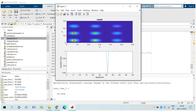
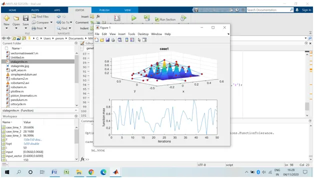
Use the toc command to deduct the run time for each and every case. You can also reduce the run time by decreasing the number of iterations.

ERRORS DURING THE PROGRAM:

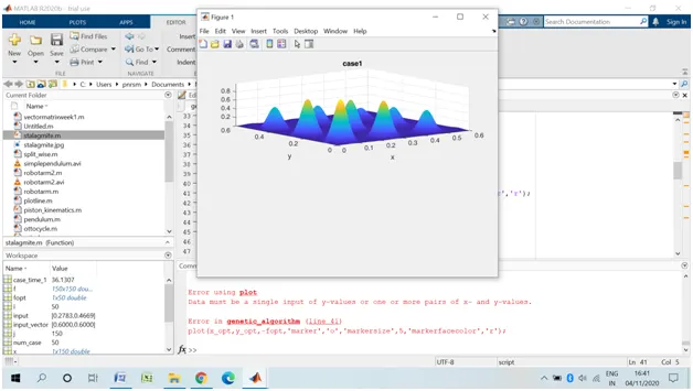
1. Use the plot3 command to create 3 axis plot. Using the PLOT command alone will display you errors in the command window and the graphical plot will not be displayed in the command window.

LEARNING OUTCOMES AND CONCLUSION:

1. We learnt on how to approach the global optimization problem using the genetic algorithm approach.

2. We also learnt on how the genetic algorithm works and its syntax.