Project-1: Modelling an electric Car with Li-ion battery

We are asked to create a MATLAB model of an electric car which uses lithium-ion battery. The major condition here is:

1. Implement the vehicle speed control using PI controller and generate brake and accelerator commands. Avoid using readymade driver block for speed control.

From this, we can understand that we cannot use the longitudinal driver block for vehicle speed control. We have to come up with a control system for speed control.

Let us look at the important steps to be followed while modeling an electric vehicle:

1. Selection of motor.

2. Motor parameters. (Rating & speed)

3. Battery pack.

4. Motor controller system.

The motor that we are going to select for this model would be the PMDC motor. PMDC stands for permanent magnet DC motor. An image of the motor is shown below.

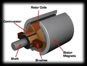
The advantage with PMDC motors is that they are highly efficient & there are no power losses. They are also smaller in size. Now we will discuss the motor rating & specifications.

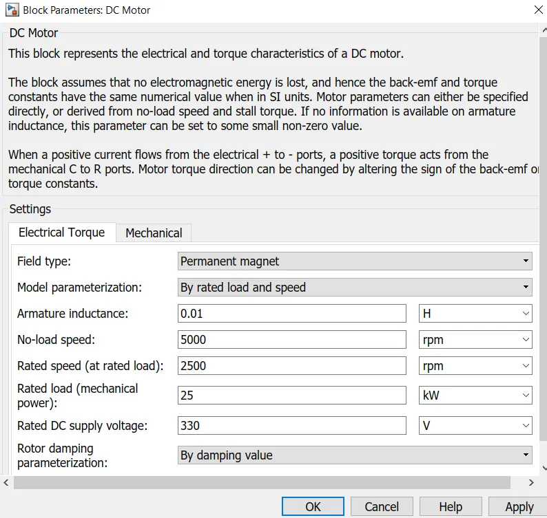
These are the rating parameters of the motor that we expect. The next would be the battery system for the motor.

We already know that lithium-ion batteries are the best source of power for EV's. The reason why everyone uses lithium ion batteries is because:

1). High energy density.

2). Compact in size.

3). Longer life.

We also have to come up with the battery voltage and current parameters for the battery pack system.

Since our PMDC motor has a supply voltage of 330V, our battery pack voltage must also provide a voltage of 330V.

The rated capacity of the battery is 75 Ah.

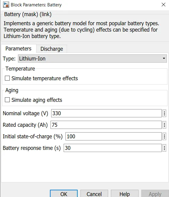
The battery parameters are also fixed. Now our motor controller is chosen.

For modeling purposes, PID & PI controllers are widely used for speed control. While modeling an EV in MATLAB, we use a reference drive cycle. After the end of modeling, we check whether our actual drive cycle matches with the reference cycle. To match them, we use PID or PI controllers.

Here, we use PI controllers. The purpose of a PI controller in a closed loop system(feedback system) is to find out the error difference. After finding out the error difference, the controller tries to negate it.

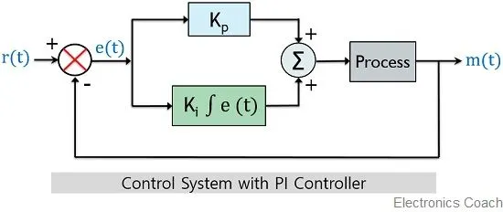
There are two controllers within the PI controller.

1. Proportional Controller:

Proportional controllers are referred as the type of controllers in which the output signal shows proportionality with the error signal. It is given as

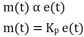
Kp is the propotional gain.

2. Integral Controller:

Integral controllers are the type of controllers where the output is proportional to the integral of the error signal. This is given as

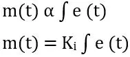
Ki is the integral gain.

The Kp & Ki gain values are the ones that minimizes the error difference in a system. These values are found out by trial and error method. We can use the Tune option in the PID tuner app in MATLAB. But since our model is not linearised(Linearised models describe the relationship between two quantities that show a constant rate of change), we cannot use the PID Tuner app.

The other motor controller that we chose is the PWM H-Bridge controller. This controller is connected to the battery pack. This H-bridge controller is used to draw only the necessary amount of current from the battery based on the EV's drive cycle speed. Using such motor controllers will help conserve energy and also control the motor speed based on the acceleration and brake commands given by the driver.

Now that our selection is done, we will look at our MATLAB model.

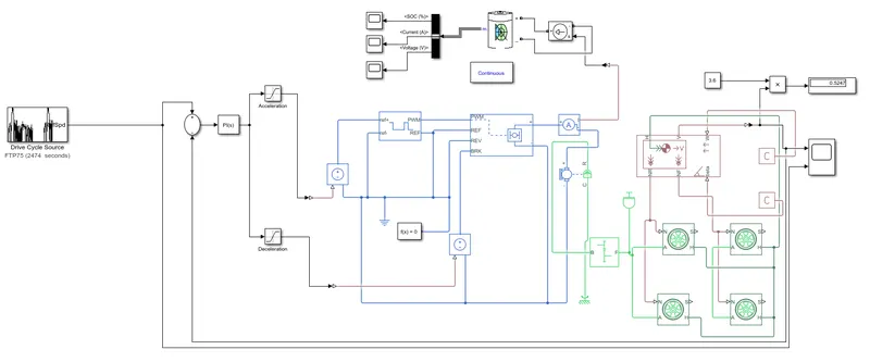
We will look at our model in detail.

DRIVE CYCLE SOURCE:

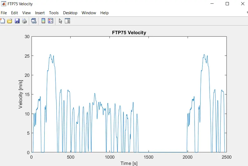
This is the reference drive cycle that we set for our EV model. This can be done using the drive cycle source block in MATLAB. Our reference drive cycle is the FTP-75 drive cycle(Federal Test Procedure).

The drive cycle plot is shown below. This plot will be our reference. The actual drive cycle should be atleast matching with the plot below.

Now we will setup a control system for the model.

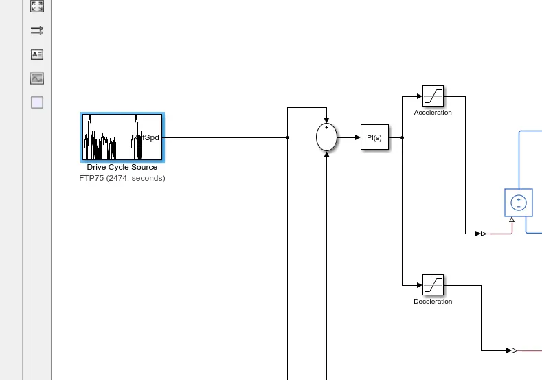
The reference drive cycle is passed onto the adder block. Then the PI controller is connected with the block. The signals coming out of the PI controller are then connected to two saturation blocks, which sets an upper & lower limit. These two signals act as the acceleration & brake commands for the EV.

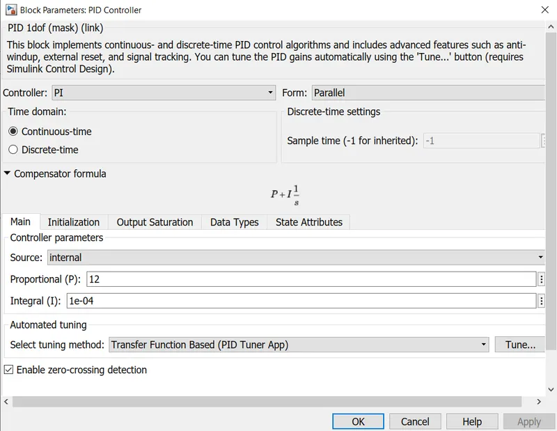
The parameters of the PI controller blocks are shown below.

Note that the values of P & I are found using trial and error method.

The saturation block parameters are seen below.

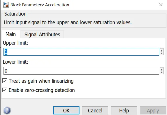
For deceleration, the upper limit is zero & lower limit is -1.

Now we will look at the H-bridge motor controller circuit.

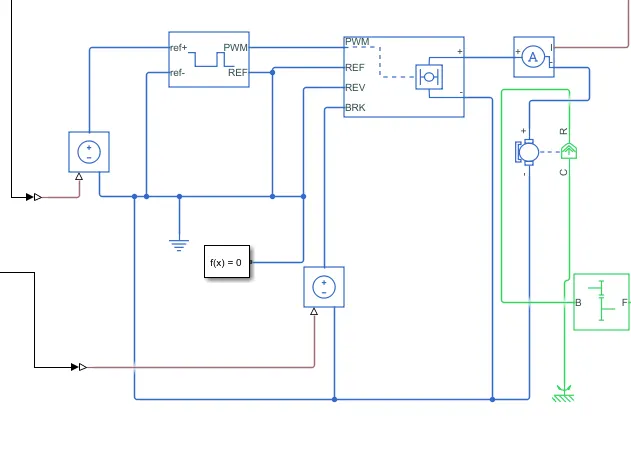
The signals coming out of the saturation blocks are sent to controlled voltage sources. The controlled voltage source block is used for the sources. They are used to keep the voltage of the signals constant regardless of the current flowing through the circuit.

Then, they are sent to a controlled PWM voltage block. This represents a pulse width modulated voltage source. The parameters of the PWM block is shown below:

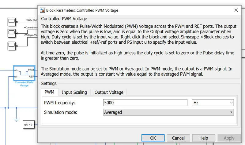
The frequecy is kept high at 5000hz. The mode of simulation is kept as averaged so as to speed up the simulation time.

Connect the voltage sources with the Controlled PWM block as shown above.

Now the H-bridge block is used. The parameters of the controller are shown below.

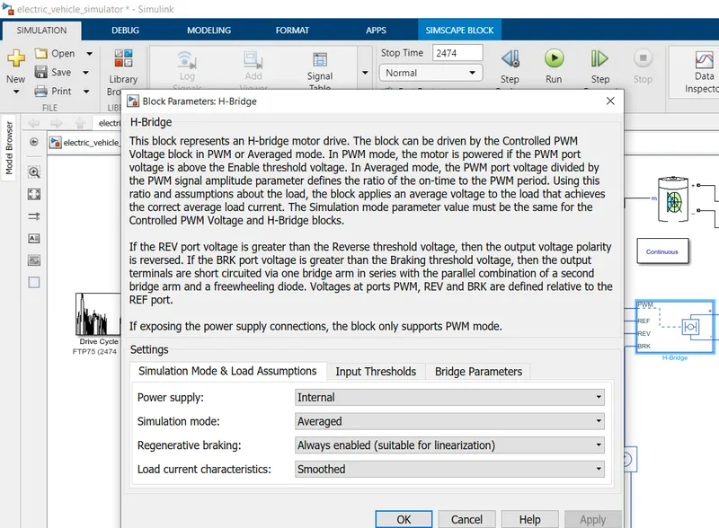
Enable the averaged simulation mode here, and also enable regenerative braking. The threshold voltage parameters are also shown below:

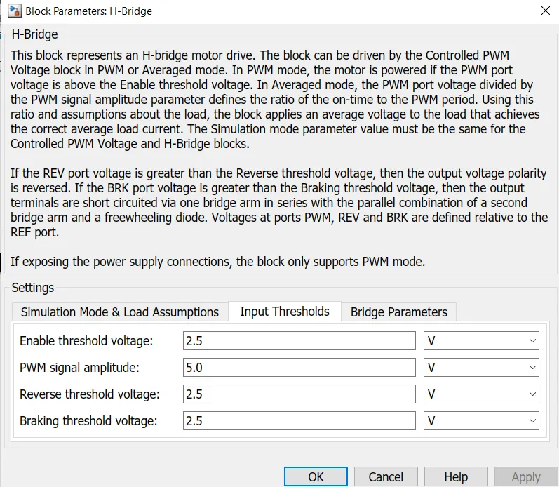
The H-bridge controller is used to change the polarity of the voltage applied at the DC motor so as to run the vehicle in forward & reverse direction as per the acceleration & brake commands.

This is the end of the controller circuit. In MATLAB, an electrical circuit must have atleast one electrical reference block & one solver configuration block connected.

Connect them anywhere in the controller circuit.

Now we will move on to the battery pack system.

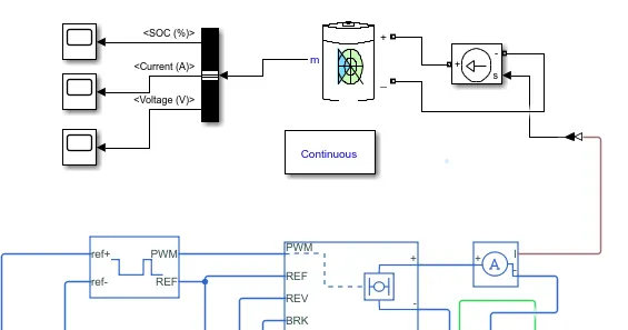
The H-bridge block is connected to a current sensor and the current sensor is connected to a controlled current source block. The generic battery block is used to create a battery pack for the model. The current sensor gives us the current entering into the controller system from the battery pack.

The battery parameters are seen below:

Now we need to extract the output from this battery. The output of this battery is the current, voltage & SOC. They can be extracted using a bus selector. The bus selector block parameters are shown below:

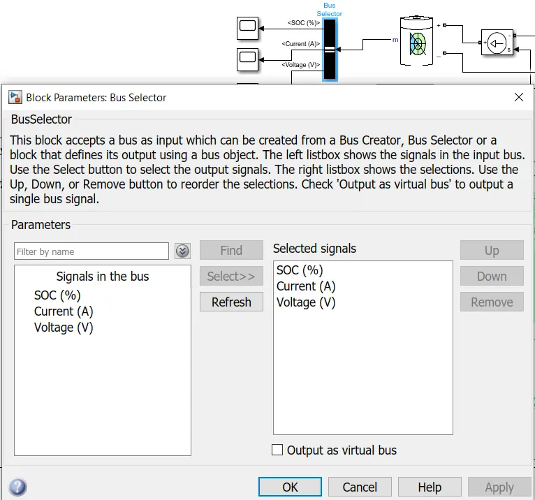
These signals are then connected to a scope window. The scope block will plot the values of current, voltage & SOC for the entire drive cycle.

Now we will see the motor drive and vehicle body system of this model.

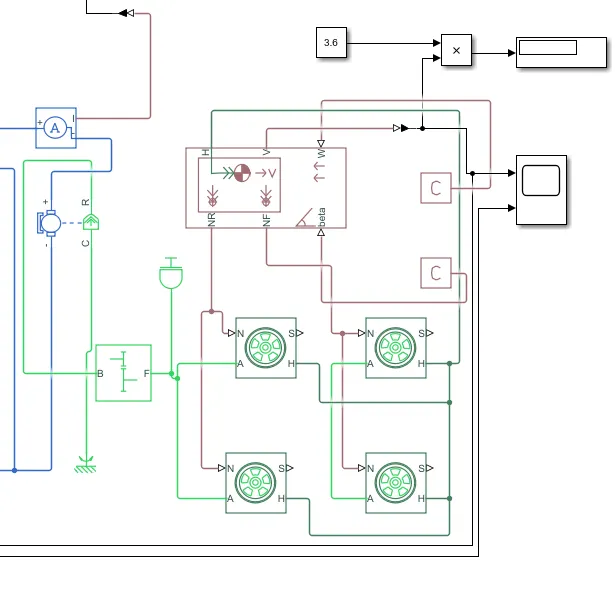
The PMDC motor is connected with the H-bridge controller, so that the motor operates based on the acceleration & brake commands given by the driver.

A mechanical rotational reference is connected to the DC motor.

The parameters of the PMDC motor is already shown above.

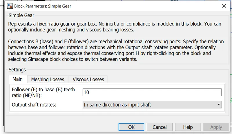
The simple gear box block is used to transmit the power from the motor to the wheels. It's parameters are shown below.

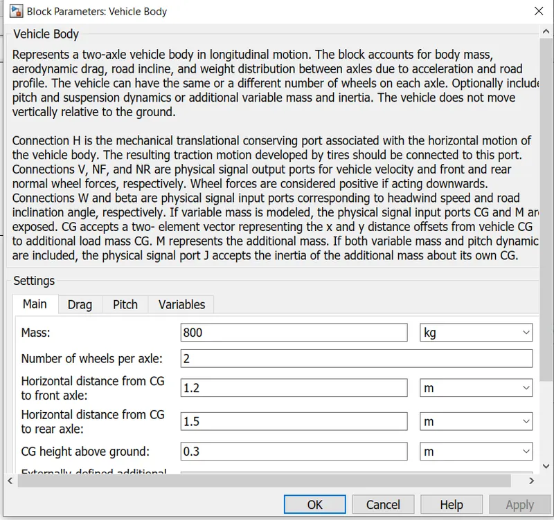
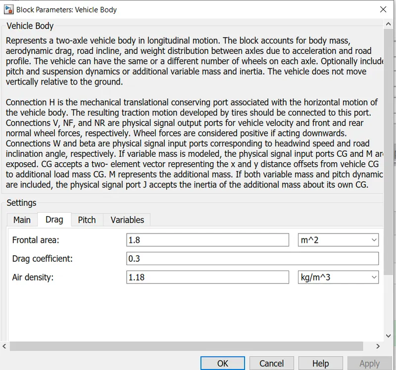
The vehicle dynamics block is used to simulate a vehicle body based on the mass, frontal area, drag co-efficient, grade angle & wind velocity etc. This is the main body of the vehicle.

The parameters are shown below.

The drag coefficient, frontal area & other parameters are shown below.

The wind velocity & the grade angle are keyed in the dynamics block using a PS constant block. Connect the PS constant block at port W for wind velocity & beta for grade angle.

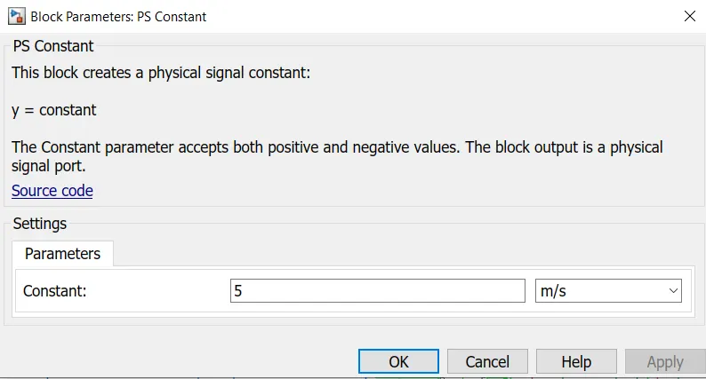
The wind velocity is kept at 5 m/s, whereas we have not considered any grade angle for the vehicle.

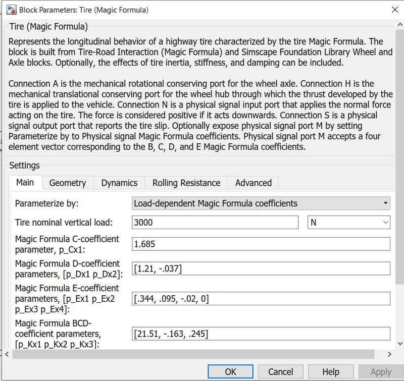
After the vehicle dynamics block, use the tire(magic formula) block to simulate the tires and connect them to the vehicle dynamics block as shown in the screenshot above.

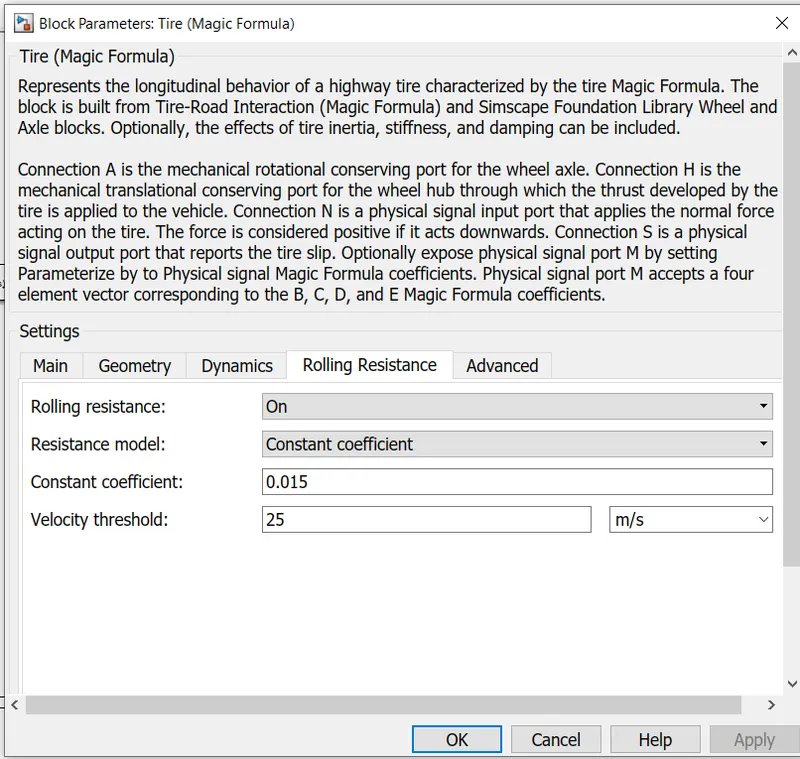
Consider the rolling resistance for the tires. The parameters of the tires are shown below.

The rolling resistance parameters are shown below.

Now use the output port of the vehicle dynamics block(the V port) to connect it to a scope window. This will help us to plot the actual drive cycle of the model.

The output of the vehicle dynamics block is fedback to the control system adder block. Doing this will minimize the error difference between the actual and reference drive cycle.

In addition, a display block is connected to the output of the vehicle dynamics block to display the speed in Kmph.

Use the constant block and convert the value from m/s. (Multiply 3.6 with velocity to get speed in kmph)

Now the model is ready for simulation.

RESULTS:

The run time is kept at 2474 seconds because the total run time of the FTP drive cycle is 2474 seconds.

Now we will see the actual drive cycle and the reference drive cycle.

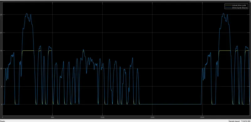
From the plot it is evident that the actual drive cycle is almost matching with the reference drive cycle.

But the peak velocity is lesser in the actual drive cycle(15m/s). This is because of many factors. The rolling resistance of the vehicle is taken into consideration & hence this will affect the velocity of the vehicle.

The wind velocity also affects the speed of the vehicle.

The SOC plot is shown below.

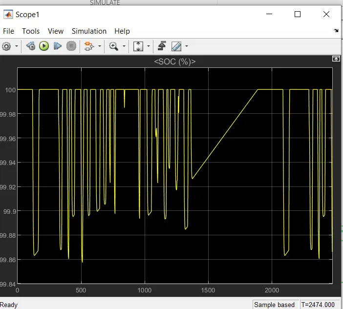
The battery SOC falls only upto 99.86%. This is because of regenerative braking. When we decelerate, the battery gets recharged. The motor functions as an electric generator during this period.

So while acceleration, the battery discharges & while deceleration, the battery charges.

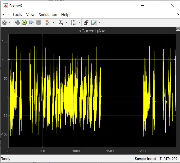
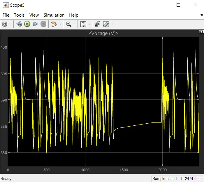
The voltage & current plots of the battery are also shown below.

CONCLUSION:

Thus we have created a MATLAB model of an EV, without using any in-built driver blocks for speed control.

The actual drive cycle had a peak velocity of 15m/s, while the reference had a peak velocity of 25m/s. This might be due to rolling resistance and wind velocity.