Project 1 - Parsing NASA thermodynamic data

AIM:

1. To write a function that extracts the 14 different temperature co-efficients through the given data. (NASA thermodynamic data).

2. To calculate the thermodynamic properties such as enthalpy, entropy and specific heat capacity from the given NASA thermodynamic data and to store them as images in different folders.

3. To also calculate the molecular weight for every species present in the data and to dispaly them in the command window.

4. To plot the specific heat capacity, enthalpy and entropy for the local temperature range.

INTRODUCTION:

1. File parsing means reading in a data stream of some sort and building an in memory model of the semantic content of that data. This aims at facilitating perfoming some kind of transformation on the data. In other words, file parsing means breaking down the given complex data in a manner that is understandable to the user.

2. In this project, we are given a file that contains thermodynamic data of different species (compounds) and we have to evaluate the thermodynamic properties from that given data. Those thermodynamic properties include:

Enthalpy: It is a measure of the heat absorbed or the heat rejected from the system.

Entropy: It is the measure of disorder or randomness in a system.

Specific heat capacity: It is the amount of heat required to raise the temperature of 1kg of a body through unit degree C.

All these properties are calculated with the help of high & low temperature co-efficients. It will be explained in detail in the function program.

3. After that, we will have to calculate the molecular weight of every single species and display it in the command window. We also have to plot the specific heat capacity, enthalpy and entropy for the local temperature range.

Now let us look at the program codes and their explanations in detail.

PROCEDURE:

1. The main program code is given below:

clear all
close all
clc

% Entering Gas constant
R = 8.314;

% File opening and reading
f1 = fopen('THERMO.dat','r')
f2 = fopen('M.weight','w')
header = fgetl(f1)

% Reading global temperature
l1 = fgetl(f1);

% For omitting lines
for i = 1:3
    l2 = fgetl(f1)
end

T = linspace(300,1000,200)

for i = 1:52
    l3 = fgetl(f1);
    A = strsplit(l3,' ');
    
    species = strtok(l3,' ');
    
    % Extracting the species coefficients in 3 lines
    a = fgetl(f1);
    b = fgetl(f1);
    c = fgetl(f1);
    
    % Position of E 
    d = strfind(a, 'E');
    e = strfind(b, 'E');
    f = strfind(c, 'E');
    
    % Extracting high temperature coefficients
    a1 = str2double(a(1:d(1)+3));
    a2 = str2double(a(d(1)+4:d(2)+3));
    a3 = str2double(a(d(2)+4:d(3)+3));
    a4 = str2double(a(d(3)+4:d(4)+3));
    a5 = str2double(a(d(4)+4:d(5)+3));
    a6 = str2double(b(1:e(1)+3));
    a7 = str2double(b(e(1)+4:e(2)+3));
    
    % Extracting low temperature coefficients
    b1 = str2double(b(e(2)+4:e(3)+3));
    b2 = str2double(b(e(3)+4:e(4)+3));
    b3 = str2double(b(e(4)+4:e(5)+3));
    b4 = str2double(c(1:f(1)+3));
    b5 = str2double(c(f(1)+4:e(2)+3));
    b6 = str2double(c(f(2)+4:e(3)+3));
    b7 = str2double(c(f(3)+4:e(4)+3));
    
    % Entering specific heat,enthalpy,entropy and molecular weight
    [CP] = specificheat(a1,a2,a3,a4,a5,b1,b2,b3,b4,b5,T,R);
    [H] = enthalpy(a1,a2,a3,a4,a5,a6,b1,b2,b3,b4,b5,b6,T,R);
    [S] = entropy(a1,a2,a3,a4,a5,a6,a7,b1,b2,b3,b4,b5,b6,b7,T,R);
    [MW] = mol_wt(species);
    
    % Species folder
    mkdir(species);
    current_dir = pwd;
    cd(species)
    
    % Plots
    % Temperature vs specific heat
    figure(1)
    plot(T,CP);
    xlabel('Temperature[k]');
    ylabel('Specific heat[KJ]');
    title('Temperature vs specific heat');
    image = getframe(gcf);
    imwrite(image.cdata,'T vs CP.png')
    saveas(1,'specific heat','jpg')
    
    % Temperature vs enthalpy
    figure(2)
    plot(T,H);
    xlabel('Temperature[k]');
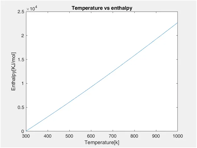
    ylabel('Enthalpy[KJ/mol]');
    title('Temperature vs enthalpy');
    image = getframe(gcf);
    imwrite(image.cdata,'T vs H.png')
    saveas(1,'enthalpy','jpg')
    
    % Temperature vs entropy
    figure(3)
    plot(T,S);
    xlabel('Temperature[k]');
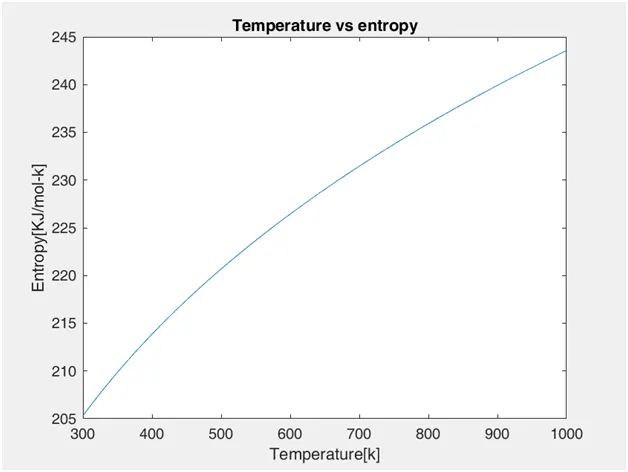
    ylabel('Entropy[KJ/mol-k]');
    title('Temperature vs entropy');
    image = getframe(gcf);
    imwrite(image.cdata,'T vs S.png')
    saveas(1,'entropy','jpg')
    
    % Change the current folder
    cd(current_dir);
    
    fprintf(f2,'Molecular weight of %s is %f n',species,MW);
end

fclose(f2);
fclose(f1);

CODE EXPLANATION:

1. Start the program with clear all, close all & clc to clear our workspace and command window.

2. Enter the value of R (Universal gas constant) as 8.314. This constant is essential in calculating the thermodynamic properties.

3. Download the thermodynamic data file before starting the program and save it in your directory.

4. Use the FOPEN command to read the data into MATLAB.

5. The 'r' notation denotes reading the file while the 'w' notation is used to write text in the file.

6. The HEADER command is used to read the initial lines of the data file.

7. Use the for loop to omit lines. There might be some unnecessary data in the file and we can go past it. In the above program, the first three lines are omitted.

8. Use the LINSPACE command to specify the local temperature range. Here, the range is from 300-1000 with 200 values in between.

9. The next step is the reading of the species and it is done using the for loop.

10. Use the STRSPLIT command here to split strings.

11. After splitting strings, we have to extract the tempreature co-efficients. Use the FGETL command for extraction.

12. We first have to find the position of the variable 'E'. Use the STRFIND command to find the position.

13. Inorder to extract the temperature co-efficients, we have to convert the strings into numerical arrays. We can use either the STR2NUM command or the STR2DOUBLE command. In the program there are 14 temperature co-efficients and we have extracted them and stored in variable groups a & b. (Ranges from a1 to a7 & b1 to b7)

14. We have used the STR2DOUBLE command since it converts text in string to double decimal precision values.

15. The co-efficients a1 to a7 are high-temperature co-efficients and b1 to b7 are low temperature co-efficients.

16. Now let us move on to evaluating the thermodynamic properties such as enthalpy, entropy and specific heat. The formulae are already given to us and it is given below:

17. We can create functions for enthalpy, entropy and specific heat so that it will be easier for us to reuse the codes into the main program. Given below are the function programs for the three thermodynamic properties:

function [CP] = specificheat(a1,a2,a3,a4,a5,b1,b2,b3,b4,b5,T,R);
t = 1000
if T > t
    CP = (a1 + a2.*T + a3.*T.^2 + a4.*T.^3 + a5.*T.^4).*R;
else
    CP = (b1 + b2.*T + b3.*T.^2 + b4.*T.^3 + b5.*T.^4).*R;
end

function [H] = enthalpy(a1,a2,a3,a4,a5,a6,b1,b2,b3,b4,b5,b6,T,R);
t = 1000;
if T > t
    H = (a1.*T + (a2.*T.^2)./2 + (a3.*T.^3)./3 + (a4.*T.^4)./4 + (a5.*T.^5)./5 + a6).*R
else
    H = (b1.*T + (b2.*T.^2)./2 + (b3.*T.^3)./3 + (b4.*T.^4)./4 + (b5.*T.^5)./5 + b6).*R
end

function [S] = entropy(a1,a2,a3,a4,a5,a6,a7,b1,b2,b3,b4,b5,b6,b7,T,R);
t = 1000
if T > t
    S = (a1.*log(T) + a2.*T + a3.*(T.^2)./2 + a4.*(T.^3)./3 + a5.*(T.^4)./4 + a7).*R
else
    S = (b1.*log(T) + b2.*T + b3.*(T.^2)./2 + b4.*(T.^3)./3 + b5.*(T.^4)./4 + b7).*R
end

18. In the function, we introduce the variable,'t' inorder to differentiate the high and low temperatures. We set the t value to 1000 and create an if-else condition. If the 't' value is less than 1000 use the coefficients a1 to a7, else use b1 to b7.

19. Call the function into the main program to evaluate the thermodynamic properties.

20. Now the next step is to find the molecular weight. We can also create a seperate function for that and it is given below:

function [MW] = mol_wt(species);
elements = ['H','O','C','N','A'];
atomic_weight = [1,16,12,14,40];
MW = 0;

% Atomic number addition

for i = 1:length(species)
    for j = 1:length(elements)
        
        if strcmpi(species(i),elements(j))==1
            
            MW = MW + atomic_weight(j)
            position = j;
        end
    end
    
    n = str2num(species(i));
    if n > 1
        MW = MW+atomic_weight(position)*(n-1);
    end
end

disp(['Molecular weight of',species,'is']);
disp(MW)

end

21. We use the for loop to include every single species and elements. We also specify the atomic weight of the basic elements.

22. We use the STRCMPI to compare the string case. We then key in the formula of the molecular weight into the loop as follows:

MW = MW + atomic weight(position)*(n-1)

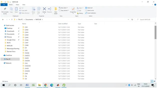
23. We then create a sperate directory and folder for each and every single species. We use the MKDIR command to create new folder or directory and 'cd' command is used to change the working directory.

24. Use the IMAGE command, SAVEAS command and IMWRITE command to save the plots as images. After running the code, when you go to the created directory, you will find the plots of each and every species in their respective folders.

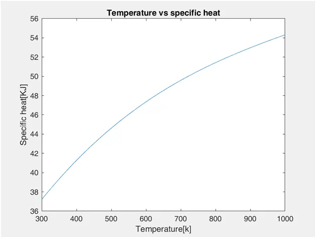
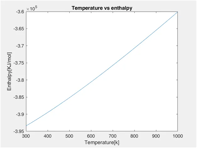
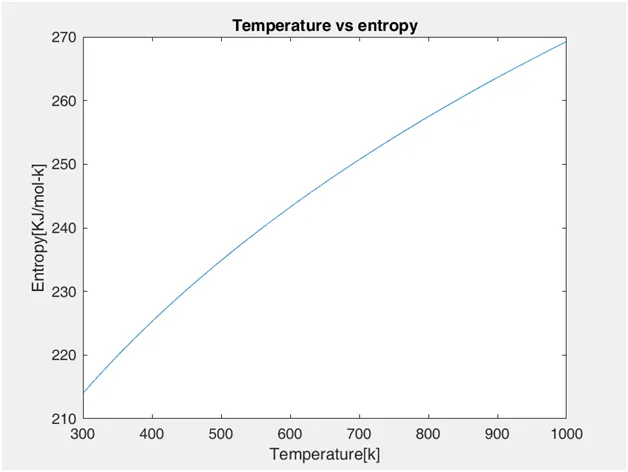
25. We now plot the thermodynamic properties calculated along with the temperatures. Use the PLOT command and FIGURE command to create plots for the three different properties.

26. In the end use the FPRINTF command to display the calculated molecular weight into the command window.

OUTPUTS:

1. Using the MKDIR command we have created folder for each and every species. Below is an attached photo:

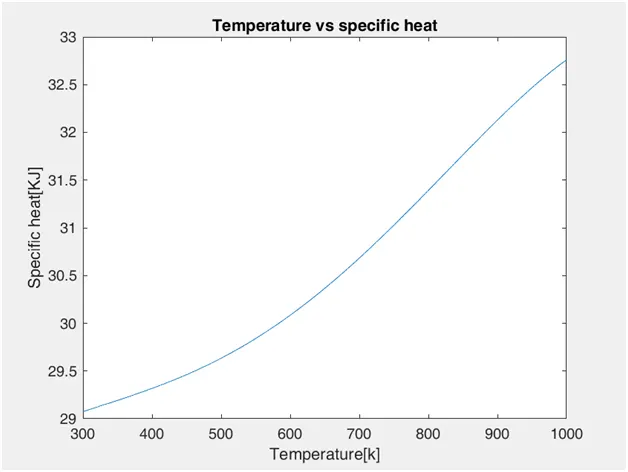
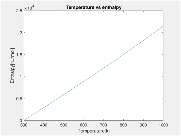
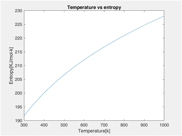
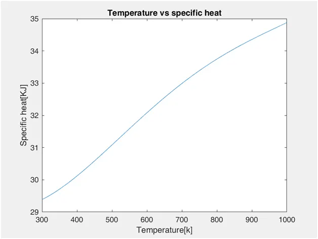
2. The plots for all species are done. For a sample reference we have attached the plot of Carbon-di-oxide, nitrogen and oxygen:

CARBON-DI-OXIDE:

NITROGEN(N2):

OXYGEN(O2):

LEARNING OUTCOMES AND CONCLUSION:

1. We have learnt the basics of file parsing using various string commands.

2. We also learnt on how to create seperate folders and directories in MATLAB using the MKDIR command.

3. We also calculated the thermodynamic and the molecular weights of the species.