Week 3 - Solving second order ODEs

AIM:

1. To solve the second order ODE of a simple pendulum.

2. To also simulate the simple pendulum for the given values of angular velocity, displacement, length, mass and damping coefficient.

INTRODUCTION:

1. ODE's represent the change in behaviour of a system with respect to time. They are of utmost importance in the engineering field to determine solutions, which will be easier for us to simulate.

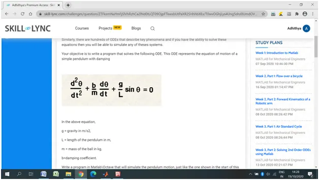
2. The governing ODE of the simple pendulum is given below:

3. Here the given example is a simple pendulum, which we have to simulate for the given values:

damping coefficient = 0.05. gravity = 9.81m/s2

length = 1m. mass = 1g. angular displacement = 0 at t = 0.

time span = 20sec. angular velocity = 3 rad/s at t = 0sec.

4. We also have to create a time plot and create an animation video which shows the oscillation of the simple pendulum for a time span of 20 seconds.

PROCEDURE:

1. The program code for the simple pendulum is given below

clear all
close all
clc

% Inputs
b = 0.05;
g = 9.81;
l = 1;
m = 1;

% Initial constraints
theta_0 = [0;3];

% Time points
t_span = linspace(0,20,500);

% ODE solver
[t,results] = ode45(@(t,theta) ode_func(t,theta,b,g,l,m),t_span,theta_0);

plot(t,results(:,1))
hold on
plot(t,results(:,2))
xlabel('time')
ylabel('plot')

% Simulation of pendulum
figure
ct = 1;
for i = 1:length(results(:,1))
    x0 = 0;
    y0 = 0;
    x1 = l*sin(results(i,1));
    y1 = -l*cos(results(i,1));
    plot([-0.5,0.5],[0,0],'linewidth',3,'color','r');
    line([x0 x1],[y0 y1],'linewidth',3,'color','b');
    hold on
    plot(x1,y1,'o','markers',30,'markerfacecolor','y');
    axis([-1.5 1.5 -1.5 0.5]);
    pause(0.03)
    grid on
    hold off
    M(ct) = getframe(gcf);
    ct =ct + 1;
end

% animation video
movie(M)
videofile = VideoWriter('simplependulum.avi','uncompressed AVI')
open(videofile)
writeVideo(videofile,M)
close(videofile)

CODE EXPLANATION:

1. Enter the input variables of the program. (b = 0.05, m = 1, l = 1, g = 9.81).

2. Now create an array (theta_0), which stores the initial values of angular displacement and angular velocity.

3. Create another array (time_span). Use the LINSPACE command to create 500 different values of time starting from 0 to 20.

4. Now let us look at how to solve the ODE. Use the command ODE45 to solve the ODE. ODE45 is an inbuilt solver in MATLAB which uses the RUNGE-KUTTA method to solve differential equation. Create a function (ode_func) to reuse the ODE program into this main program. The code of the function ode_func is given below:

function [dtheta_dt] = ode_func(t,theta,b,g,l,m)

theta1 = theta(1)
theta2 = theta(2)
dtheta1_dt = theta2;
dtheta2_dt = -(b/m)*theta2 - (g/l)*sin(theta1);
dtheta_dt = [dtheta1_dt ; dtheta2_dt];
end

5. After succesfully inserting the function, we will get our solution to the ODE. The solution should be stored as an array [t, results], which is a 500x2 matrix. It has 500 different solutions for angular displacement and angular velocity since our time span input had 500 different values. This is enough to create a time plot.

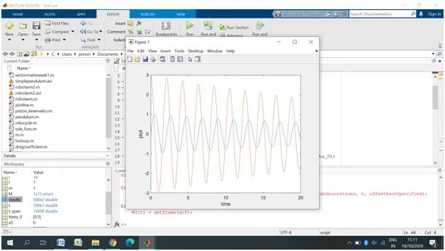
6. Use the PLOT function to create a time graph. The x-axis will specify the time and the y-axis will specify the angular displacement and angular velocity. Below is the attached photo.

Now let us proceed to the simulation of the simple pendulum.

7. A simple pendulum will be looking like this.

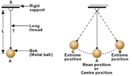
It will have a rigid support. A thread will be suspended from that support and a bob is tied to the free end of the string. We have to simulate like this exactly in the graph.

8. We can create this with the help of the FOR LOOP. And we can use the MOVIE command to create an animation file of the simple pendulum.

9. We must first determine the range ie., the number of times the FOR LOOP needs to be executed. We need to simulate the pendulum for all values of angular displacement. Hence the range of the FOR LOOP would be,

for i = 1: length(results(;,1)).

10. The initial co-ordinates are set as x0 = 0 and y0 = 0. The counter variable (ct) is set to an initial value of 1 before the commencement of the FOR LOOP execution. This is to avoid overlapping of plots.

11. Now let us plot the rigid support. Since the support is fixed, use the co-ordinates x = -0.5 0.5 and y = 0 0 as the points for the support. Use the PLOT function, and create the thickness for the rigid support using the LINEWIDTH command. (Ideal width is 3).

12. Now we need to find the length of the string during oscillations. We already have our length of the string at mean position as 1m and we have the values of angular displacement for different values of time. Hence the formula is given as :

x1 = l*sin(results(i,1)) y1 = -l*cos(results(i,1)) since the string is suspended downwards.

Use the PLOT command and specify the co-ordinates as (x0,x1) (y0,y1). Enter the linewidth value as 3. Use the HOLD ON command so that these plots do not get erased.

13. Now the bob has to be simulated. Use the MARKERS function to simulate the bob as a sphere. The center position of the bob would be x1 and y1. Apply them in the PLOT function. You can also give a color to the bob using the MARKERFACECOLOR command.

14. Use the AXIS command to specify the limits for the plot. Turn on the grids using the GRID ON command. Use the PAUSE command to change the time interval for two different plots in an animation.

15. Use the GETFRAME command at the end of the FOR LOOP to capture all the frames we obtained with the help of the FOR LOOP. Also use the MOVIE command outside the FOR LOOP to create a video file format.

16. This is how you would simulate a simple pendulum. The animation video is attached below as a google drive link for reference.

https://drive.google.com/file/d/1IBcD6dhJbsQ8vujcpE1Zv4sYtTFQTTEK/view?usp=sharing

LEARNING OUTCOMES AND CONCLUSION:

1. We learnt on ODE's and its applications in the field of engineering

2. We also learnt on how to simulate a simple pendulum and create a time plot.