Week-4 Challenge WOT Condition Part-2

QUESTION 1:

1. What is the difference between mapped and dynamic model of engine, motor and generator? How can you change model type?

First let us look at what is the difference between mapped model and dynamic model.

MAPPED MODEL:

This model uses a set of steady-state lookup tables to characterize engine performance.

The tables provide overall engine characteristics, including actual torque, fuel flow rate, BSFC, and engine-out exhaust emissions.

Some examples of when one should use mapped models are:

1. When you have engine data from a dynamometer or a design tool like GT-POWER.

2. For quasi steady-state engine simulations.

This model will have a lesser simulation time because the data points are already assigned in lookup tables. Lesser accuracy when compared to the dynamic model.

DYNAMIC MODEL:

This model decomposes the engine behavior into engine characteristics that are separated into lower-level components. By combining components in this way, the models capture the dynamic effects.

Given below are some instances when dynamic models are applied:

1. If you need a more detailed dynamic model and have component-level data.

2. To analyze the impact of individual engine components on the overall performance.

Higher simulation time because each and every individual component is analysed for the overall performance of the system. But the accuracy is a lot better.

How can one change the model type:

1. Go to the POWERTRAIN blockset module in MATLAB. Select any reference vehicle model. For example, we have selected the EV reference application blockset. Its block diagram is shown below.

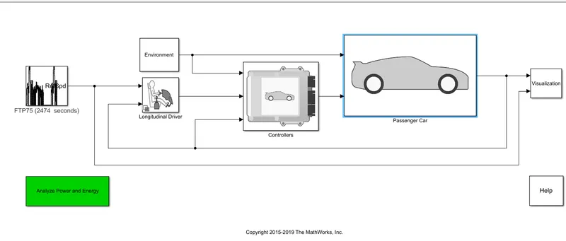
2. Now double click on the PASSENGER CAR block. Inside that block there will be an ELECTRIC PLANT block. Click on that block to view the contents inside.

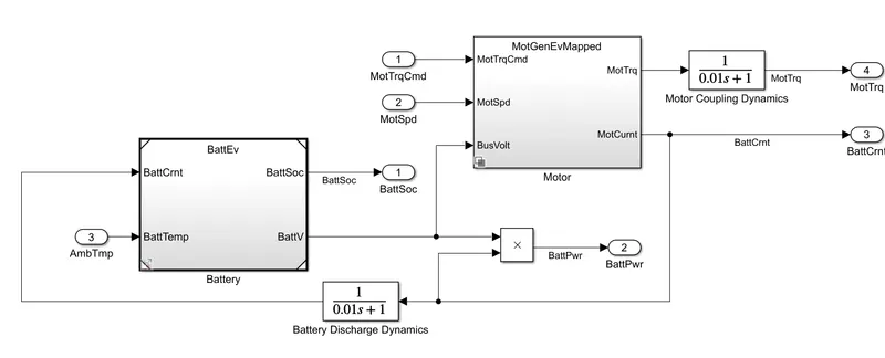
These are the contents inside that block. In the motor block as you can see the model is set as a mapped model. In order to change that into a dynamic model, just right click on that block and select VARIANT-LABEL MODEL ACTIVE CHOICE. Now you can set that model into dynamic. The screenshot is displayed below for better understanding.

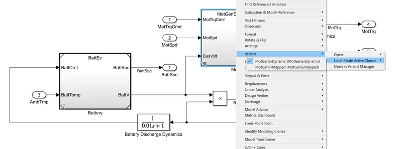
This is how one can change the mapped model into a dynamic model and vice versa.

QUSETION 2:

2. How does the model calculate miles per gallon? Which factors are considered to model fuel flow?

Miles per gallon is a fuel economy rating followed in some countries in order to estabish a relationship between fuel consumed and distance travelled by the vehicle. It is the distance travelled by a vehicle for one gallon of fuel. (1 gallon = 4 litres approx).

In the POWERTRAIN blockset the fuel economy is calculated as follows:

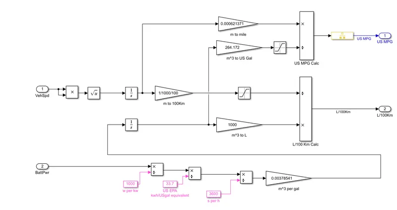
Open any vehicle model available in the POWERTRAIN blockset module. Here we have opened the performance calculations block of an electric vehicle.

VEHICLE SPEED:

Here our fuel in this case is the battery pack. The model considers the vehicle speed, which is the drive cycle input here and the battery power of the vehicle to calculate the fuel economy.

In the vehicle speed, we can see that there is conversion happening. When we integrate speed with time, we get distance. This distance is converted from m into 100kms as well as miles and fed into two blocks, L/100 and the USMPG block. (In the US, the MPG is calculated for miles). (1m = 0.000621 miles).

We are measuring the amount of litres of fuel (in this case equivalent battery power) required to travel for 100 kms. And also the distance covered for USMPG. Then these results are compared.

BATTERY POWER:

The initial battery power is in Watts and it is converted into KW(Dividing by 1000). Then power is converted into energy by multipying with time. Then we convert energy into eqivalent energy in US gallons (Dividing energy with 33.7).

Then we further divide it by 3600 to convert KWh into KWs. Then we have to convert it to volume of fuel flow. The fuel flow unit is m^3/gallon and it has to be multiplied by a factor of 0.00378541 with the energy value. This fuel flow is further integrated to convert it in to m^3. It is multiplied by 1000 to convert it into litres. This is fed into the L/100kms block.

Then it is also converted into equivalent US gallons by multiplying m^3 units to 264.172. This is fed into the US MPG block.

Then the integrated distance measured is converted into miles and fed into the US MPG block. It is again converted to 100kms and fed to the L/100kms block. These results are then used for comparison.

Finally, the distance measured and the energy flow are calculated and they are divided to get the result in miles/gallon.

This is how the miles per gallon calculation is done in the powertrain blockset.

QUESTION 3:

3. Run the HEV Reference Application with WOT drive cycle. Change the grade and wind velocity in the environment block. Comment on the results.

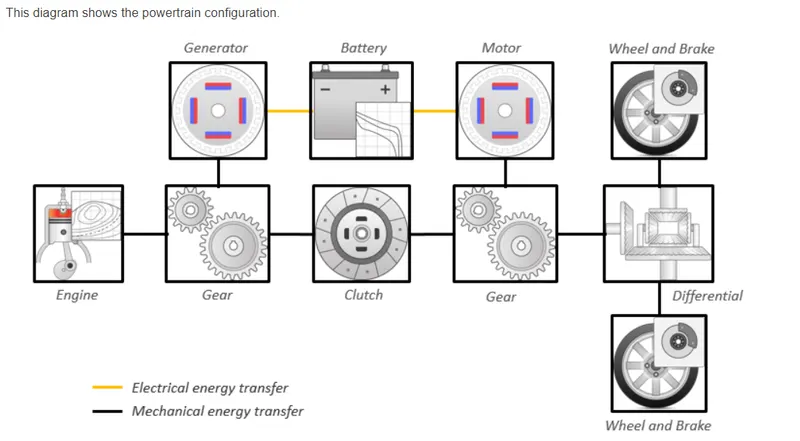
The HEV uses both ICE(Internal Combustion engine) and a battery propulsion system to move a vehicle. The powertrain sequence of a HEV is shown below for a better understanding on how the powertrain is transmitted.

Now let us look at the block diagram setup of a HEV.

Open the HEV reference application using the MATLAB documentation. The block diagram is shown below.

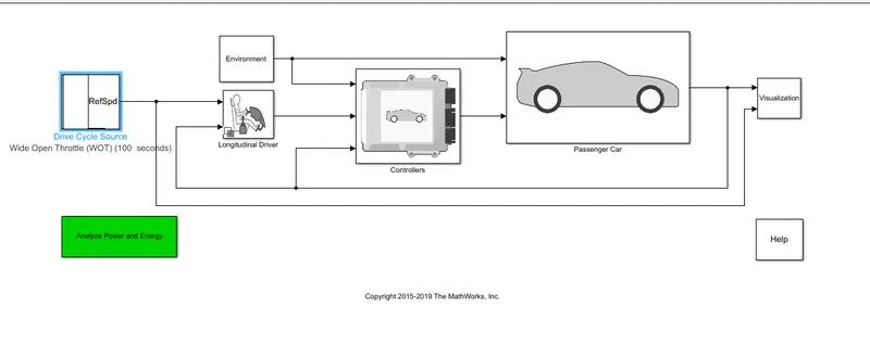
Here we have converted the drive cycle from FTP 75 to WOT drive cycle. The specifications are shown below:

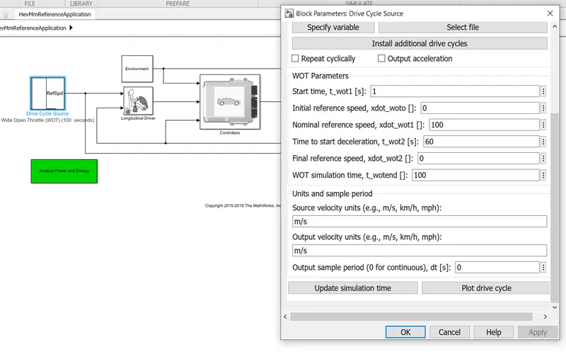
Start time = 1s. Initial speed = 0mph. Final speed = 100mph. Time to start deceleration = 60s. WOT time = 100s.

Now we have to change the wind velocity and grade as well. Go to the ENVIRONMENT block to apply grade and wind velocity. The block diagram is shown below.

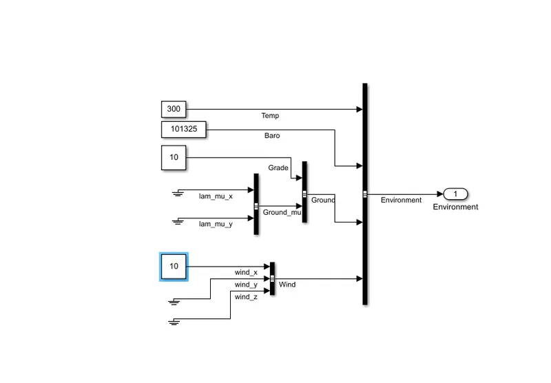
We have applied the grade angle as 10 degrees and the wind speed as 10 m/s.

Now we can run the performance tests and view the results. Run the system for a stop time of 100 secs.

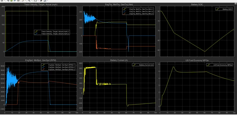
The first plot shows us the target velocity graph and the actual velocity. We wanted the maximum speed to be 100mph but because of the grade angle, wind velocity the max speed acheived was only 60 mph.

The acceleration time from initial to maximum speed was approximately close to 60 secs and the deceleration time from max. to min was found to be 5 secs approximately.

The second plot shows us the speeds of motor, generator and engine. From the plots, it is evident that the RPM is considerably greater while the vehicle is accelerating and lower when decelerating.

The third plot shows us the torque for the motor, engine and generator. We can observe the same pattern as the torque is high while acceleration and low when deceleration.

The fourth plot shows us the battery current in ampere. The current flow is clearly high when the vehicle is at the accelerating period and it decreases sharply during deceleration.

The fifth plot shows us the SOC of the battery during the WOT cycle. The SOC depletes during acceleration and gradually increases during deceleration and also due to the regenerative braking.

The final plot shows us the fuel economy as USMPG. The economy is clearly higher when the vehicle is battery driven. But it starts to decrease when IC engine starts to drive the vehicle.

From these results we can clearly say that environmental factors impact the overall performance of the vehicle. If the wind velocity and grade angle were lesser, the performance would have been more enhanced.

QUESTION 4:

4. Keeping all other parameters same, compare the simulated results of hybrid and pure electric powertrains.

A pure EV uses only a battery propulsion system to run a vehicle. The powertrain setup of a pure EV is shown below.

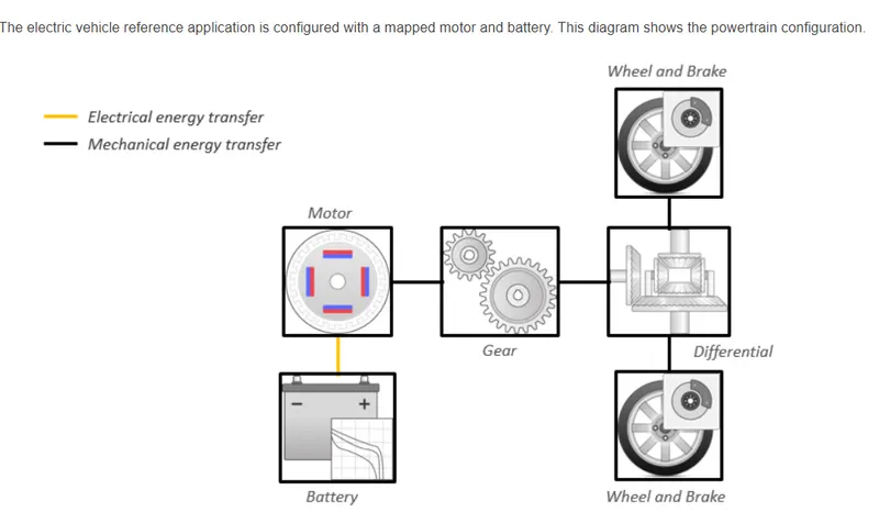
Since we have already discussed about the performance of the HEV above, we will look into the performance of a pure EV with the same input parameters.

The block diagram setup of a pure EV is opened using the MATLAB documentation.

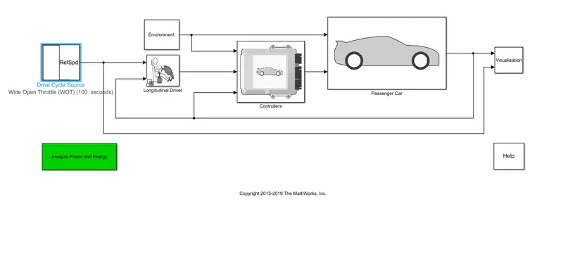
The same WOT drive cycle is followed.(Refer the HEV WOT drive cycle above). The same environmental drive conditions are set. ( Wind velocity = 10 m/s. Grade angle = 10 degrees.)

Now run the system for a stop time of 100 secs. The results are attached below.

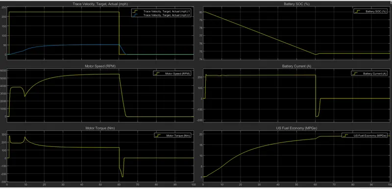
The first plot shows us the target velocity graph and the actual velocity of the EV. We wanted the EV to acheive a maximum speed of 100 mph, but the actual drive cycle shows a max. velocity of 51.7 mph. This might be due to the environmental conditions.

The second plot shows us the motor speed in RPM. It is evident that the RPM is high during acceleration and low during deceleration.

The third plot shows us the motor torque in N-m. The same pattern follows, the torque is high for higher speeds and low during deceleration.

The fourth plot shows us the SOC during different speeds and time. The SOC was initially at 80% and drops down to approximately 75%. It further increases because of regenerative braking.

The fifth plot shows us the battery current in ampere. Higher speeds require higher current, so the current is higher initially and it drops down for lower speeds.

The final plot shows us the fuel economy. The economy continuously increases since we dont have any engines and generators.

So from this we can conclude that a pure EV is better than HEV because:

1. Lesser SOC decline. With the same input parameters, we saw a decline upto 58% in HEV's, but in a pure EV the decline was only till 75%.

2. Better fuel economy. The MPG value was found to be higher for a pure EV than a HEV.

3. Zero emissions in the case of a pure EV. Since we use ICE in a HEV, emissions are produced.