Week 4.1 - Genetic Algorithm

                                                                                                                                    Report

in this project i used MATLAB to optimise the stalagmite function and find the global maxima of the function.

generally optimization concept used to minimize or maximize the perticular function.and stalagmite function used to generate local minima or local maxima.and genetic algorithm ,first introduced by holland is a powerful stochastic search algorithm based on the mechanism of natural genetic and selection.general description of GA is as follows:

genetic algorithm cycle:

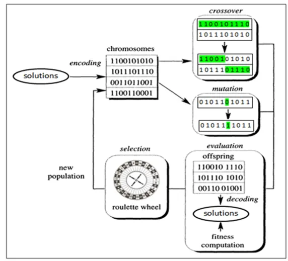
• genetic algorithm start with an initial set of random solution called population. 
• each individual in the population is called a chromosome representing a solution to the problem at hand.
• the chromosomes evolve through successive iiiteration called generation.
• during each generation the chromosomes are evaluuated using some measures of fitness.
• to create the next generation new chromosomes called offspring are formed by either merging two chromosomes from current generation using a crossover operator or modifying a chromosome using a mutation operator.
• a new generation is formed by selecting according to the fitness value some of the parents and offspring and rejecting others so as to keep the population size constant
• filter chromosomes have higher probabilities of being selected
• after several generation the algorithm converge to the best chromosomes which hopefully representes the optimum or suboptimal solution to the problem.

genetic algorithm syntex used in matlab : 

x= ga(fun,nvars,A,b,Aeq,beq,lb,ub,nonlcon,intcon,options)

fun = Objective function, specified as a function handle or function name. Write the objective function to accept a row vector of length nvars and return a scalar value.

nvars = Number of variables, specified as a positive integer. The solver passes row vectors of length nvars to fun.

A = Linear inequality constraints, specified as a real matrix. A is an M-by-nvars matrix, where M is the number of inequalities.

b = Linear inequality constraints, specified as a real vector. b is an M-element vector related to the A matrix. If you pass b as a row vector, solvers internally convert b to the column vector b(:)

Aeq = Linear equality constraints, specified as a real matrix. Aeq is an Me-by-nvars matrix, where Me is the number of equalities.

beq = Linear equality constraints, specified as a real vector. beq is an Me-element vector related to the Aeq matrix. If you pass beq as a row vector, solvers internally convert beq to the column vector beq(:).

lb = Lower bounds, specified as a real vector or array of doubles. lb represents the lower bounds element-wise in lb ≤ x ≤ ub.Internally, ga converts an array lb to the vector lb(:).

ub= Upper bounds, specified as a real vector or array of doubles. ub represents the upper bounds element-wise in lb ≤ x ≤ ub.Internally, ga converts an array ub to the vector ub(:).

nonlcon = Nonlinear constraints, specified as a function handle or function name. nonlcon is a function that accepts a vector or array x and returns two arrays, c(x) and ceq(x).

intcon = Integer variables, specified as a vector of positive integers taking values from 1 to nvars Each value in intcon represents an x component that is integer-valued.

options = Optimization options, specified as the output of optimoptions or a structure.

% defining our workspace
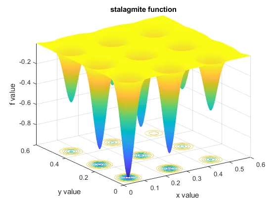
x = linspace(0,0.6,150);
y = linspace(0,0.6,150);
iterations = 50;

% creating 2 diamensional mesh
[xx,yy] = meshgrid(x,y);

% evaluating stalagmite function

for i = 1:length(xx)
   for j = 1:length(yy)
    input_vector(1) = xx(i,j);
    input_vector(2) = yy(i,j);
    f(i,j) = stalagmite_func(input_vector);
   end
end
figure(1)
surfc(xx,yy,f)
shading interp
xlabel('x value')
ylabel('y value')
zlabel('f value')
title('stalagmite function')

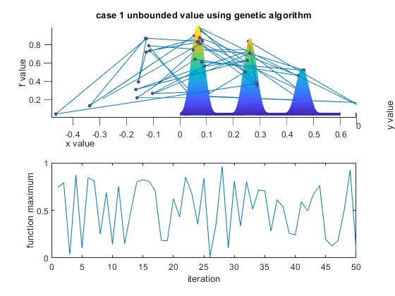
% case 1 unbounded value using genetic algorithm
tic
for i = 1:iterations
    [inputs,fop1(i)] = ga(@stalagmite_func,2);
    xop1(i) = inputs(1);
    yop1(i) = inputs(2);
end
case1_t=toc
figure(2)
subplot(2,1,1)
hold on
surfc(xx,yy,-f)
shading interp
xlabel('x value')
ylabel('y value')
zlabel('f value')
title('case 1 unbounded value using genetic algorithm')
plot3(xop1,yop1,-fop1,'marker','o','MarkerSize',3,'MarkerFaceColor','r')
subplot(2,1,2)
plot(-fop1)
xlabel('iteration')
ylabel('function maximum')
global_max1 = -fop1


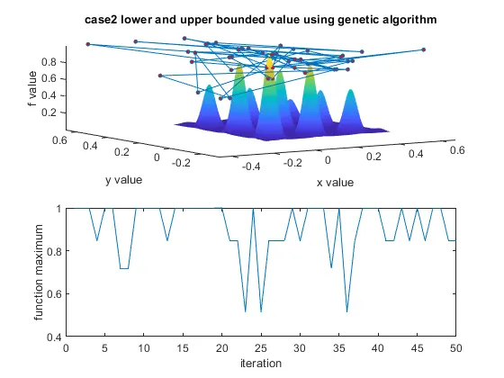
% case2 = lower and upper bounded value using ga

tic
for i= 1:iterations
    [inputs,fop2(i)] = ga(@stalagmite_func,2,[],[],[],[],[0;0],[1;1]);
    xop2(i)=inputs(1);
    yop2(i)=inputs(2);
end
case2_t=toc

figure(3)
subplot(2,1,1)
hold on
surfc(xx,yy,-f)
shading interp
xlabel('x value')
ylabel('y value')
zlabel('f value')
title('case2 lower and upper bounded value using genetic algorithm')
plot3(xop1,yop1,-fop2,'marker','o','MarkerSize',3,'MarkerFaceColor','r')
subplot(2,1,2)
plot(-fop2)
xlabel('iteration')
ylabel('function maximum')
global_max2 = -fop2

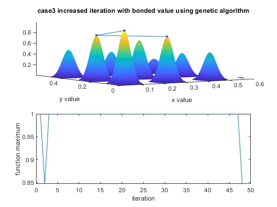
% case3 increased iteration with bonded value using ga
options = optimoptions('ga')
options = optimoptions(options,'populationsize',170);

tic
for i= 1:iterations
    [inputs,fop3(i)] = ga(@stalagmite_func,2,[],[],[],[],[0;0],[1;1],[],[],options);
    xop3(i)=inputs(1);
    yop3(i)=inputs(2);
end
case3_t=toc
figure(4)
subplot(2,1,1)
hold on
surfc(xx,yy,-f)
shading interp
xlabel('x value')
ylabel('y value')
title('case3 increased iteration with bonded value using genetic algorithm')
plot3(xop3,yop3,-fop3,'marker','o','MarkerSize',3,'MarkerFaceColor','r')
subplot(2,1,2)
plot(-fop3)
xlabel('iteration')
ylabel('function maximum')
global_max3 = -fop3