Project 2 - Rankine cycle Simulator

Report

Aim:

To simulate the rankine cycle and plot the T-S and H-S diagram using MATLAB.

Objective:

• Create a Rankine Cycle Simulator using MATLAB.
• calculate the state points of the Rankine Cycle (any type of your choice) based on user inputs.
• Then, plot the corresponding T-s and h-s plots for the given set of inputs.

Given Inputs:

Turbine Inlet temperature = 400° C

Turbine Inlet Pressure = 30 bars

Turbine Outlet Pressure = 0.05 bars = Condenser Inlet Pressure

Required outputs:

1] Net work output

2] Back work ratio

Notes:

The standard Xsteam library is usd to get the steam table data for water, is given. It must be used to calculate the points in between the state variables.

Introduction:

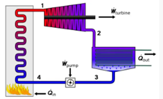
• 1-2 : isentropic expansion in turbine
• 2-3 : constant pressure heat rejection at condenser
• 3-4 : isentropic compression in pump
• 4-1 : constant pressure heat addition at boiler

• Rankine cycle is used in steam power plant.in this working fluid change its phase during cycle.in this cycle we use water is working fluid.
• In rankine cycle essential components are pump,boiler,turbine,condenser.pump is used to increasses the pressure of water at constant volume.and boiler is used to heat addition process. in boiler water is converted into super heated steam and this super heated steam is passed on turbine to produce required output.after that condenser is used to reduce dryness fraction of steam.so steam expand upto low temperature due to which turbine work and efficiency of steam power plant is increasses.
• if rankine cycle is compared to carnot cycle then observation show that the rankine cycle have maximum work ratio and back work ratio is low and specific steam consumption [SSC]also low. specific steam consumption means rate of mass of steam required to produce unit output power.work ratio means ratio of net work output to positive work.and back work ratio means the ratio of negative work to positive work.
• in order to increases the efficiency of rankine cycle we can use re-heating and regeneration technique.

Design criteria of rankine cycle:

• boiler pressure selected such way that the quality of steam at exit of turbine is high.
• condensor pressure decided by cooling water temperature,its means condensor pressure selected such way that saturation temperature must be greater then the cooling water temperature.
• superheating of steam in boiler is depend on material properties of system.

Basic model of rankine cycle:

• 1-2 : isentropic expansion in turbine
• 2-3 : constant pressure heat rejection at condenser
• 3-4 : isentropic compression in pump
• 4-1 : constant pressure heat addition at boiler

MATLAB program:

clear all
close all
clc
fprintf('RANKINE CYCLE \n')
fprintf('1-2 : isentropic expansion in turbine \n')
fprintf('2-3 : constant pressure heat rejection at condenser \n')
fprintf('3-4 : isentropic compression in pump \n')
fprintf('4-1 : constant pressure heat addition at boiler \n ')



% user inputs
P1 = input('enter the boiler pressure[bar]:');
P2 = input('enter the condensor pressure[bar]:');
T1 = input('enter the turbine inlet temperature[degree celsius]:');

%state point 1

H1 = XSteam('h_pt',P1,T1); 
S1 = XSteam('s_pt',P1,T1);
Hf1 = XSteam('hL_p',P1);
Hg1 = XSteam('hV_p',P1);
Ts1 = XSteam('Tsat_p',P1);
Sf1 = XSteam('sL_p',P1);
Sg1 = XSteam('sV_p',P1);

% state point 2

S2 = S1;
Sf2 = XSteam('sL_p',P2);
Sg2 = XSteam('sV_p',P2);
x = (S2-Sf2)/(Sg2-Sf2);
Hf2 = XSteam('hL_p',P2);
Hg2 = XSteam('hV_p',P2);
H2 = Hf2 + x*(Hg2-Hf2);
T2 = XSteam('Tsat_p',P2);
Ts2 = XSteam('Tsat_p',P2);

% state point 3

H3 = Hf2;
S3 = Sf2;
T3 = T2;
P3 = P2;

% state point 4

P4 = P1;
S4 = S3;
H4 = XSteam('h_ps',P4,S4);
T4 = XSteam('T_ph',P2,H2);

% temperature value for plotting saturation curve
t = linspace(0,374,500);

% plot saturation curve
for i = 1:length(t)
    a(i) =XSteam('sV_T',t(i));
    b(i) =XSteam('hV_T',t(i));
    c(i) =XSteam('sL_T',t(i));
    d(i) =XSteam('hL_T',t(i));
end
% plot T-S diagram
figure(1)
% plot rankine cycle
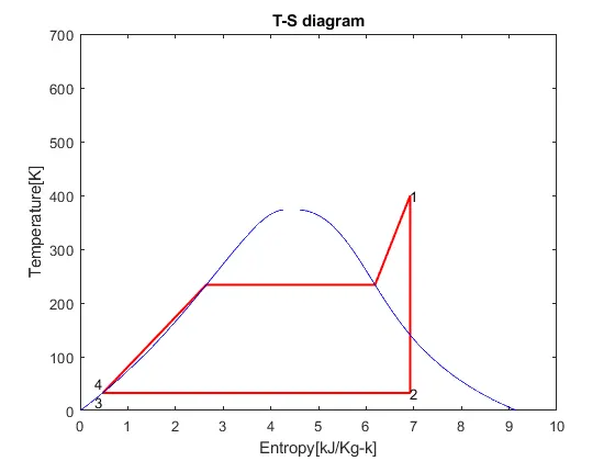
plot([S1 S2 S3 S4 Sf1 Sg1 S1],[T1 T2 T3 T4 Ts1 Ts1 T1],'LineWidth',1.5,'Color','r')
hold on
% plot saturation curve
plot(c,t,'Color','b')
plot(a,t,'Color','b')
axis([0 10 0 700])
text(S1,T1,'1','FontSize',10)
text(S2,T2,'2','FontSize',10)
text(S3,T3,'3','FontSize',10,'HorizontalAlignment','right','VerticalAlignment','top')
text(S4,T4,'4','FontSize',10,'HorizontalAlignment','right','VerticalAlignment','bottom')
xlabel ('Entropy[kJ/Kg-k]')
ylabel('Temperature[K]')
title('T-S diagram')

% plot H-S diagram
% plot rankine cycle
figure(2)
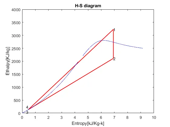
plot([S1 S2 S3 S4 S1],[H1 H2 H3 H4 H1],"LineWidth",1.5,"Color",'r')
axis([0 10 0 4000])
hold on
% plot saturation curve
plot(a,b,'Color','b')
plot(c,d,'Color','b')
text(S1,H1,'1','FontSize',10)
text(S2,H2,'2','FontSize',10)
text(S3,H3,'3','FontSize',10,'HorizontalAlignment','right','VerticalAlignment','top')
text(S4,H4,'4','FontSize',10,'HorizontalAlignment','right','VerticalAlignment','bottom')
xlabel ('Entropy[kJ/Kg-k]')
ylabel('Ethalpy[KJ/kg]')
title('H-S diagram')

% calculation

% turbine work
WT = H1-H2;
% pump work
WP = H4-H3;
% heat addition
Qin = H1-H4;
% heat rejection
Qout = H2-H3;
% net work
Wnet = WT-WP;
% efficiency
thermal_efficiency = (Wnet/Qin)*100;
% specific steam consumption
SSC = 3600/Wnet;
% back work ratio
BWR = WP/WT;

% ALL RESULT
fprintf('RESULT \n')
fprintf('At state point 1 : \n')
fprintf('P1 is : %.3f bar \n',P1)
fprintf('T1 is : %.3f degree celsius \n',T1)
fprintf('H1 is : %.3f KJ/Kg \n',H1)
fprintf('S1 is : %.3f KJ/Kg-k \n',S1)

fprintf('At state point 2 : \n')
fprintf('P2 is : %.3f bar \n',P2)
fprintf('T2 is : %.3f degree celsius \n',T2)
fprintf('H2 is : %.3f KJ/Kg \n',H2)
fprintf('S2 is : %.3f KJ/Kg-k \n',S2)

fprintf('At state point 3 : \n')
fprintf('P3 is : %.3f bar \n',P3)
fprintf('T3 is : %.3f degree celsius \n',T3)
fprintf('H3 is : %.3f KJ/Kg \n',H3)
fprintf('S3 is : %.3f KJ/Kg-k \n',S3)

fprintf('At state point 4 : \n')
fprintf('P4 is : %.3f bar \n',P4)
fprintf('T4 is : %.3f degree celsius \n',T4)
fprintf('H4 is : %.3f KJ/Kg \n',H4)
fprintf('S4 is : %.3f KJ/Kg-k \n',S4)

fprintf('SUMMERY OF ALL RESULT : \n')
fprintf('WT is : %.3f KJ/Kg \n',WT)
fprintf('WP is : %.3f KJ/Kg \n',WP)
fprintf('Qin is : %.3f KJ \n',Qin)
fprintf('Qout is : %.3f KJ \n',Qout)
fprintf('Wnet is : %.3f KJ/Kg \n',Wnet)
fprintf('thermal_efficiency is : %.3f percent \n',thermal_efficiency)
fprintf('SSC is : %.3f KJ/KWH \n',SSC)
fprintf('BWR is : %.3f \n',BWR)

explanation of code:

• programe start with clear all,close all,clc.
• after that use fprintf command to print cycle name and cycle process.
• use input command to user input such as boiler pressure,condensor pressure,temperature.
• by using xsteam function we are able to calculate the all state point of rankine cycle.
• create temperature value for plotting saturation curve by using linespace command.
• for plotting saturation curve we use the for loop.
• after that we use plot command to plotting saturation curve[in blue color] and rankine cycle[in red color] for T-S and H-S diagram.

Result:

command window:

RANKINE CYCLE 
1-2 : isentropic expansion in turbine 
2-3 : constant pressure heat rejection at condenser 
3-4 : isentropic compression in pump 
4-1 : constant pressure heat addition at boiler 
 enter the boiler pressure[bar]:30
enter the condensor pressure[bar]:0.05
enter the turbine inlet temperature[degree celsius]:400
RESULT 
At state point 1 : 
P1 is : 30.000 bar 
T1 is : 400.000 degree celsius 
H1 is : 3231.571 KJ/Kg 
S1 is : 6.923 KJ/Kg-k 
At state point 2 : 
P2 is : 0.050 bar 
T2 is : 32.875 degree celsius 
H2 is : 2110.708 KJ/Kg 
S2 is : 6.923 KJ/Kg-k 
At state point 3 : 
P3 is : 0.050 bar 
T3 is : 32.875 degree celsius 
H3 is : 137.765 KJ/Kg 
S3 is : 0.476 KJ/Kg-k 
At state point 4 : 
P4 is : 30.000 bar 
T4 is : 32.875 degree celsius 
H4 is : 140.762 KJ/Kg 
S4 is : 0.476 KJ/Kg-k 
SUMMERY OF ALL RESULT : 
WT is : 1120.863 KJ/Kg 
WP is : 2.997 KJ/Kg 
Qin is : 3090.809 KJ 
Qout is : 1972.943 KJ 
Wnet is : 1117.866 KJ/Kg 
thermal_efficiency is : 36.167 percent 
SSC is : 3.220 KJ/KWH 
BWR is : 0.003

T-S diagram:

H-S diagram:

Errors:

no complicated errors occurred while running the MATLAB program.

conclusion:

• rankine cycle is the basic cycle for understanding about the steam turbine system in thermodynamic.
• the required output value are obtained from given input parameter.
• net work output = 1117.866 KJ/Kg
• back work ratio = 0.003
• thus the rankine cycle is successfully simulated using MATLAB.