Week 3 - Solving second order ODEs

write a program that solves the ODE that represents the equation of motion of a simple pendulum with damping.

Main program:

%input
% b=damping co-efficient(N-S/m),g=gravity(m/s^2),l=length pf pendulum(m),m=mass of
% pendulum(kg)
b = 0.1;
g = 9.81;
l = 1;
m = 1;
% initial condition:initial angular displacement=0,initial angular velocity=3
theta_0 = [0;3]
% time points
t_span = linspace(0,20,200)
% solve ODE
[t,result] = ode45(@(t,theta) ode_func(t,theta,b,g,l,m),t_span,theta_0)

figure(1)
hold on

plot(t,result(:,1),'LineWidth',1.5,'Color','r')
plot(t,result(:,2),'LineWidth',1.5,'Color','g')

xlabel('time')
ylabel('angular displacement in red color & angular velocity in green color')
title('motion of a simple pendulum with damping')
legend('angular displacement','angular velocity')

THETA = result(:,1)
ct=1;
for i=1:length(THETA)
    x0=0;
    y0=0;

    x1=-l*sin(THETA(i));
    y1=-l*cos(THETA(i));

    figure(2)
    plot([x0 x1],[y0 y1],'LineWidth',2,'Color','b')
    hold on
    plot(x0,y0,'s','Markersize',25)
    plot(x1,y1,'Marker','o','Markersize',30,'color','r')
    hold off
    xlim([-1.5,1.5])
    ylim([-1.5,1.5])
    title('motion of a simple pendulum with damping')
   
    M(ct)=getframe(gcf);
    ct=ct+1;
end
movie(M)
videofile = VideoWriter('motion_of_the_pendulum.avi','Uncompressed AVI');
videofile.FrameRate = 10
open(videofile)
writeVideo(videofile,M)
close(videofile)

Sub-program:

function [dtheta_dt] = ode_func(t,theta,b,g,l,m)
theta1 = theta(1)
theta2 = theta(2)
dtheta1_dt=theta2;
dtheta2_dt=-(b/m)*theta2-(g/l)*sin(theta1);
dtheta_dt=[dtheta1_dt;dtheta2_dt];
end

Result:.

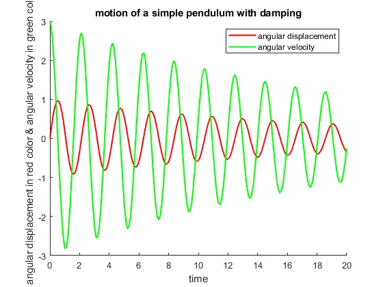
• Time vs angular displacement in red colour & angular velocity in green colour.

• youtube link of animation of simple pendulum motion : https://youtu.be/Zzur_0qY1YM

Report

this is second order ODE equation for coding perpose we need convert into two first order ODE equation.

this are two first order ODE equation:

1] dtheta1_dt=theta2;
2] dtheta2_dt=-(b/m)*theta2-(g/l)*sin(theta1);

• Step wise explanation of code.

%input
% b=damping co-efficient(N-S/m),g=gravity(m/s^2),l=length pf pendulum(m),m=mass of
% pendulum(kg)
b = 0.1;
g = 9.81;
l = 1;
m = 1;

in first step i take same input that's given in problem.in which b=damping co-efficient(N-S/m), g=gravity(m/s^2), l=length pf pendulum(m), m=mass of pendulum (kg).

% initial condition:initial angular displacement=0,initial angular velocity=3
theta_0 = [0;3]

in this step theta_0 is array variable. in this arrays 0 is initial angular displacement and 3 is initial angular velocity at time =0 which is mension in problem.

% time points
t_span = linspace(0,20,200)

in this step t_span is variable its required for integration here i divide 20 sec.in 200 equal number of part thats why we use linspace command.

function [dtheta_dt] = ode_func(t,theta,b,g,l,m)
theta1 = theta(1)
theta2 = theta(2)
dtheta1_dt=theta2;
dtheta2_dt=-(b/m)*theta2-(g/l)*sin(theta1);
dtheta_dt=[dtheta1_dt;dtheta2_dt];
end

in this step i define the ode_func function.(t,theta,b,g,l,m) this are input parameter.after that i define the theta1 and theta2 as a theta(1) and theta(2).after that [dtheta1_dt=theta2]this is the 1st ODE and [dtheta2_dt=-(b/m)*theta2-(g/l)*sin(theta1)] this is a 2nd ODE.after that we combine both ODE into array like [dtheta_dt=[dtheta1_dt;dtheta2_dt]] its coloum matrix.

% solve ODE
[t,result] = ode45(@(t,theta) ode_func(t,theta,b,g,l,m),t_span,theta_0)

in this step result are 200*2 arrays matrix and ode45 is inbuild ODE solver in matlab. @(t,theta) are the main input parameter in which t is dependant variable and theta independant variable.ode_func((t,theta,b,g,l,m)) is main function in which (t,theta,b,g,l,m) are input value.t_span is time array its used for integration to be done.theta_0 is the initial condition of system.

figure(1)
hold on

plot(t,result(:,1),'LineWidth',1.5,'Color','r')
plot(t,result(:,2),'LineWidth',1.5,'Color','g')

xlabel('time')
ylabel('angular displacement in red color & angular velocity in green color')
title('motion of a simple pendulum with damping')

legend('angular displacement','angular velocity')

in figure (1) we plot the graph between time vs angular displacement so we put the result(:,1) its mean select all row of 1st colomn and time vs angular velocity.so we put the result(:,2) its mean select all row of 2nd colomn.

THETA = result(:,1)

here we need crate animation so we need store all value of angular displacement from result 200*2 matrix.THETA is variable where all value is stored.

ct=1;
for i=1:length(THETA)
x0=0;
y0=0;

x1=-l*sin(THETA(i));
y1=-l*cos(THETA(i));

figure(2)
hold on
plot([x0 x1],[y0 y1],'LineWidth',2,'Color','b')
plot(x1,y1,'Marker','o','color','r')
title('motion of a simple pendulum with damping')

M(ct)=getframe(gcf);
ct=ct+1;
end

for animation we need to store the all angular displacement position of pendulum image and after that combine all this images for animation.so we use the FOR loop.here i=1:length(THETA)in which one by one all theta value execute. [x0,y0] is fixed point of pendulum and [x1,y1] is calculate for each angular displacement value.in figure (2) we plot the motion of a simple pendulum with damping.

M(ct)=getframe(gcf);

movie(M)
videofile = VideoWriter('motion_of_the_pendulum.avi','Uncompressed AVI');
videofile.FrameRate = 10
open(videofile)
writeVideo(videofile,M)
close(videofile)

so create animation using above code.

• Errors faced while programming :

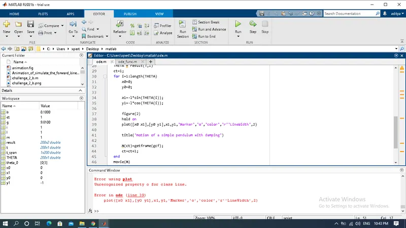
• How have you overcome those errors.

here i try to combine both plot command but we get this error so i kept as it is.

plot([x0 x1],[y0 y1],'LineWidth',2,'Color','b')
plot(x1,y1,'Marker','o','color','r')