Week 3 Challenge: DC-DC Converter

Week 3 Challenge: DC-DC Converter

1. Tune Compensator for DC Motor Using Bode Diagram Graphical Tuning

G = 1.5 / （s^2 + 14s + 40.02）

Rise time of less than 0.5 seconds, Steady-state error of less than 5%, Overshoot of less than 10%, Gain margin greater than 20 dB, Phase margin greater than 40 degrees

2. Can a system with pole on right half of the s-plane be stable? Justify your answer with an example.

3. Make a model of closed loop voltage controlled DC-DC converter. Determine suitable PI gain values to track the output voltage set point. Changing the supply voltage, load and switching frequency requires modifications in PI gain values?

1. Tune Compensator for DC Motor Using Bode Diagram Graphical Tuning -

G = 1.5 / （s^2 + 14s + 40.02）

Rise time of less than 0.5 seconds, Steady-state error of less than 5%, Overshoot of less than 10%, Gain margin greater than 20 dB, Phase margin greater than 40 degrees.

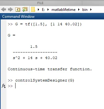
By seeing the transfer function, one can understand it is second order LTI system. The Poles and zeros determine the characteristics of the system. To find poles of system, the roots of characteristic equation must be equated to zero

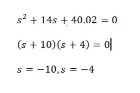
The poles are at -10 and -4 on the left side of s-plane.There is no Zero. The system is stable second order system.

Rise Time: Time taken for the system response to reach 100% of its final value for the first time.

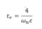
Peak Time: Time taken for the system response to reach peak value for the first time.

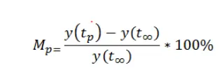
Peak Overshoot: Peak overshoot is the peak value of the response curve measured from unity.

The compensator is designed to meet the shortcomings of desired performance of the plant. To design the compensator, define the plant transfer function in MATLAB window.

Open the Control System Designer window for the defined transfer function by using controlSystemDesigner command

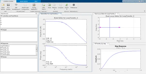
The Control system designer window displays the BODE plot editor and Root locus editor side by side along with Step response. One must tune the compensator to satisfy the condition of design requirements. On bode plot editor, the magnitude plot needs to be adjusted to around 4 rad/sec to get rise time and overshoot as per the condition.

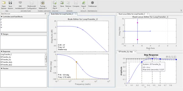
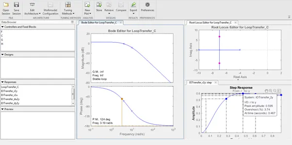
The Rise time and Overshoot have got satisfied now. To achieve 5% of steady state error, the integrator must get added by right clicking the Magnitude plot of Bode plot editor as shown below.

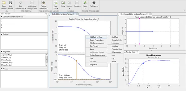
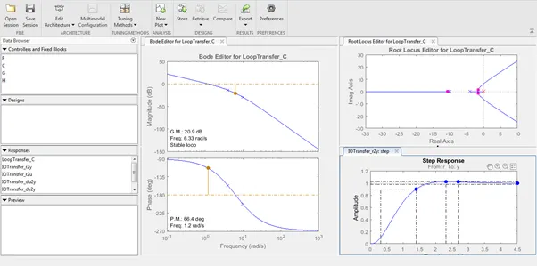
The gain of compensator is increased directly by selecting Edit compensator. We can calculate the gain value from

The gain value can be increased to 100. The lead compensator can be added with pole at -25 and zero at -5. Lead compensator will reshape the frequency-domain plot by providing sufficient phase lead angle over some appropriate frequency range to offset the excessive phase lag associated with the plant. The transfer function of lead compensator is

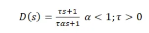
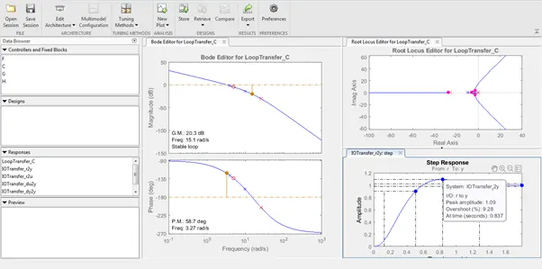
Now the design requirements have been satisfied. Hence, this is one of the ways of designing compensator to meet design requirements. One can try their own method to design the compensator.

2. Can a system with pole on right half of the s-plane be stable? Justify your answer with an example

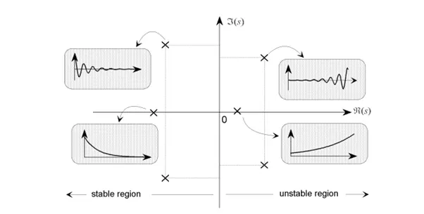
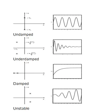
From above image we can see that poles in the right half of the S plane are unstable.

A system is said to be stable if for bounded input there exists the bounded output.

The stability of a linear system may be determined directly from its transfer function. A n^th order linear system is asymptotically stable only if all of the components in the homogeneous response from a finite set of initial conditions decay to zero as time increases, or

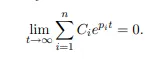
where the p_i are the system poles. In a stable system all components of the homogeneous response must decay to zero as time increases. If any pole has a positive real part there is a component in the output that increases without bound, causing the system to be unstable.

In order for a linear system to be stable, all of its poles must have negative real parts, that is they must all lie within the left-half of the s-plane. An “unstable” pole, lying in the right half of the s-plane, generates a component in the system homogeneous response that increases without bound from any finite initial conditions. A system having one or more poles lying on the imaginary axis of the s-plane has non-decaying oscillatory components in its homogeneous response, and is defined to be marginally stable.

Stability: The total response of a system is the sum of the forced and natural responses:

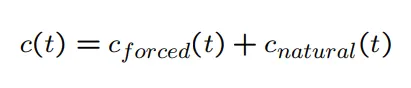
A linear, time-invariant system is stable if the natural response approached zero as time approaches infinity.

2. A linear, time-invariant system is unstable is the natural response grows without bound as time approaches infinity.
3. A linear, time-invariant system is marginally stable if the natural response neither decays or grow, but remains constant or oscillates as time approaches infinity

By looking at the placement of the poles of a system in the s-plane we can draw conclusions about the stability of a system. 1. If the poles of the closed loop are in the left half of the s-plane (negative and real), the system is stable. 2. If the poles of the closed loop are in the right half of the s-place (positive and real), the system is unstable. 3. If the poles appear on the imaginary axis and none appear in the Right Hand Plane, the system is marginally stable.

Example –

We will do Stability analysis using MATLAB Root Locus Plot –

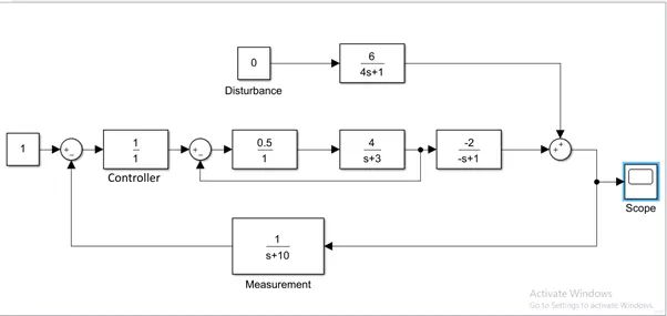
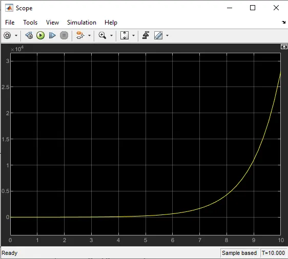
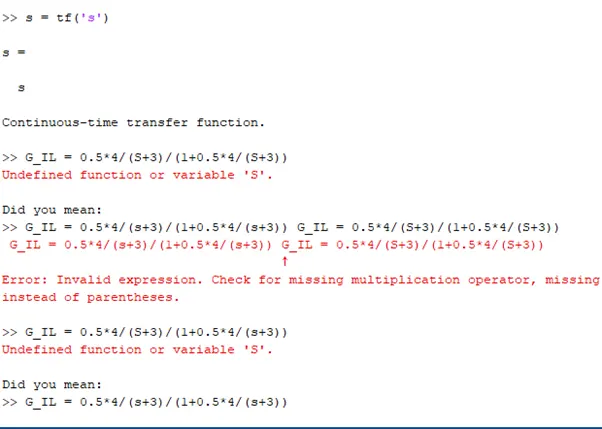
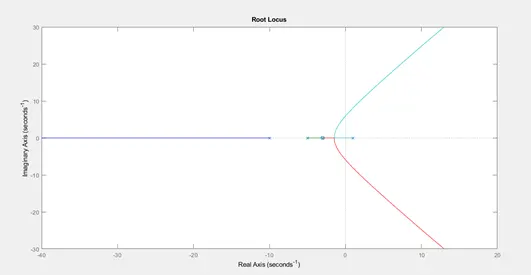
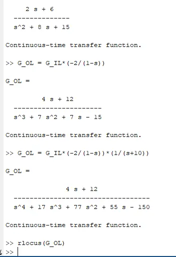
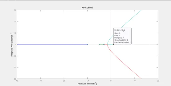
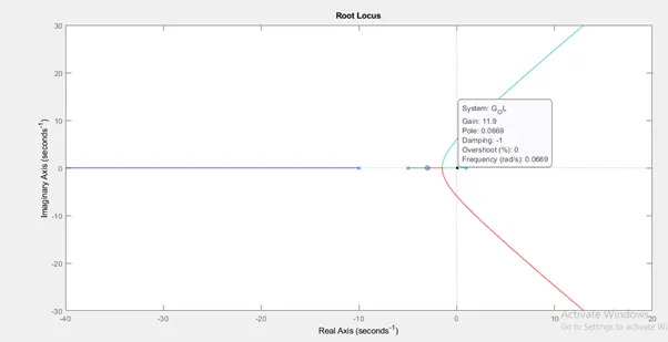
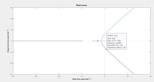
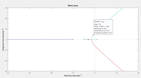
Now we will look into the Simulink System –

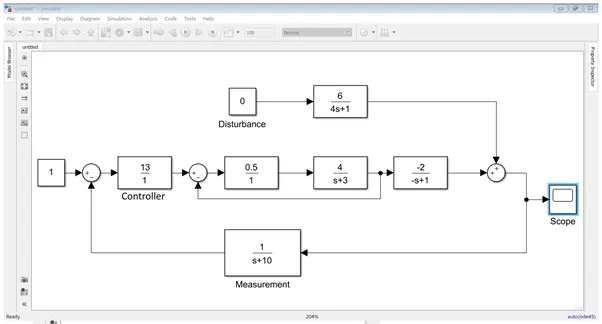
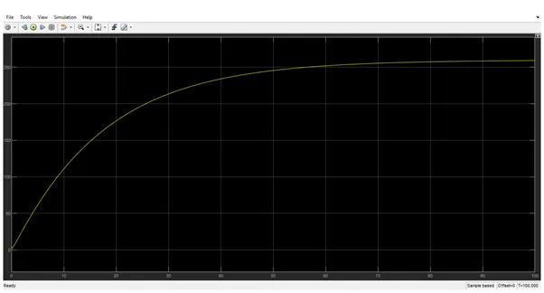
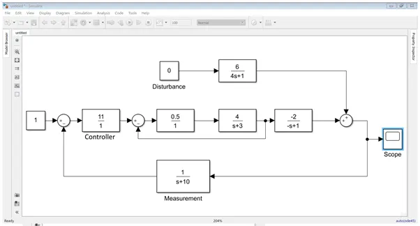
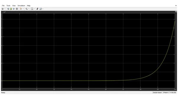
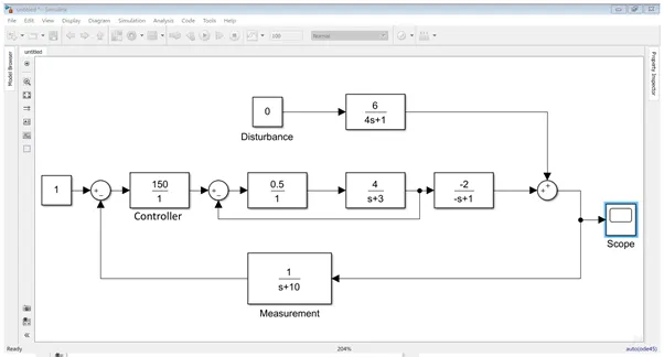
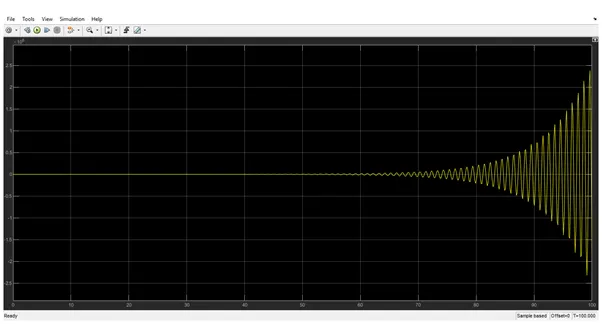
From the above plot we can see that the system is unstable and lies right half on the S – plane.

To make the system stable we will revaluate the value on the controller panel –

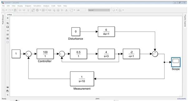
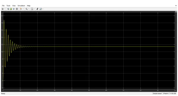
3. Make a model of closed loop voltage controlled DC-DC converter. Determine suitable PI gain values to track the output voltage set point. Changing the supply voltage, load and switching frequency requires modifications in PI gain values?

DC-DC converters have wide several applications in electrical industry, they can be employed for varied DC voltage usages and stabilization or the control of DC voltage of a battery or it can be a component of a complex converter to control the intermediate or output voltages. Due to their switching property included in their structure, DC-DC converters have a non-linear behaviour and their controlling design is accompanied with complexities. But by employing the average method it is possible to approximate the system by linear system and exploiting linear control methods. Controlling of Buck converters by method of Linear Quadratic Regulator (LQR). This method is employed for controlling Buck converter and improving its dynamic functioning, but determining the LQR controlling matrices is very difficult. So, genetic algorithm and Tabu Search, (TS), are employed to eliminate this obstacle. The simulation results show an improvement in voltage control response.

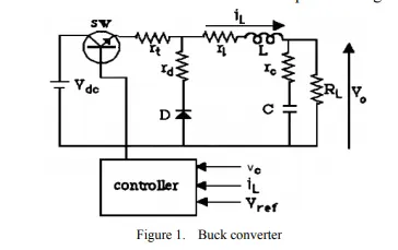
Buck converter has a wide application in electrical industry and power systems and specifically it can supply the voltage for a direct current consumer. Buck is a one input and multiple-output in structure with a non-linear property due to its switching behaviour, but at the same time when the switch is on and off its behaviour is linear. Therefore, by employing the averaging method, it is possible to exchange a non-linear system with a linear one. Many of the methods are centred on the isolation of the system variables and PI controller design. Some control methods have defined the subject of control based on pole placement. One of the other control methods is the use of feedback stage in DC converter control. Other control method is the feedback loop control. Another one is the use of LQR method in the control of Buck converter. Some control methods have stated the issue of control through pole placement. To administer different control methods, varied models of DC-DC converters are presented which have satisfactory responses. In this article an optimum LQR is designed that can improve the Buck converter response. There is no specific method in LQR design which is based on trial and error. The best constant values for state feedback matrix are laboriously obtained through trial and error, although time consuming. Genetic algorithm is employed to find the best values for LQR controller in a very short time, and also this work is done by tabu search, and get optimized matrices for LQR controller. Therefore, these new methods are presented for optimizing the systems with two factors of the least response time and the highest precision.

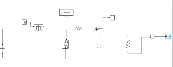
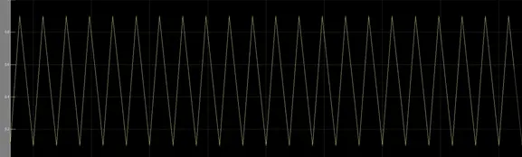
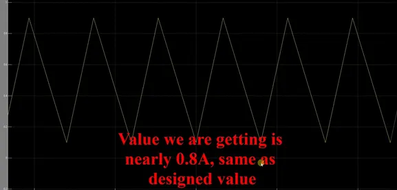
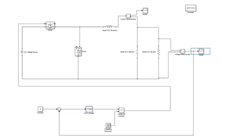
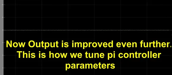
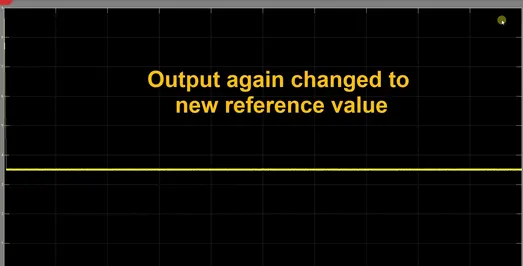
We changed PI gain values to track the output voltage set point. Changing the supply voltage, load and switching frequency requires modifications in PI gain values