PROJECT 3 – MASS SPRING DAMPER IN SIMSCAPE AND SIMULINK MODEL AND CALCULATING WORKDONE FOR GIVEN INPUT & IMPLIMENTING THE GIVEN EQUATION IN SIMULINK MODEL.

PROJECT 3 – MASS SPRING DAMPER IN SIMSCAPE AND SIMULINK MODEL AND CALCULATING WORKDONE FOR GIVEN INPUT & IMPLIMENTING THE GIVEN EQUATION IN SIMULINK MODEL

Aim-

To find work done by the cutting tool, create model to implement the given equation and analyse the example of ‘Mass Spring Damper’ using Simulink.

Objectives-

1. To determine the work done as the tool moves through the distance of 100 MM using the given data

Distance (mm)	0	20	40	60	80	100
Force (KN)	60	72	65	53	44	50

2.To implement the equation & store result values using File block.3.In Simulink open ‘MASS – Spring – Damper in Simulink & Simscape model’ and derive the governing equation for it. 3.Change the value of Mass, Damper, & Spring for the simscape system & plot the result and change the value of Mass x₀ = 2 in Simulink model and plot the results. Make the response from Simscape & Simulink as 2 separated displays.

Part 1 -

EXPLANATION –

Workdone-

W = F * D

W = workdone in Nm.

F = Force.

D = Design (m).

Work is said to be done when an object moves (displaces) along the direction of appliacation of force.

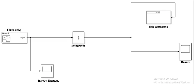
Signal Builder Block Graph –

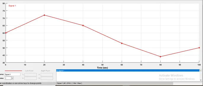
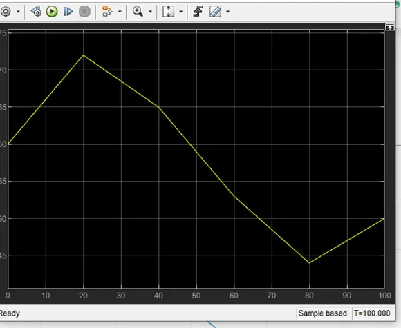
A plot of Force vs. Distance is given below-

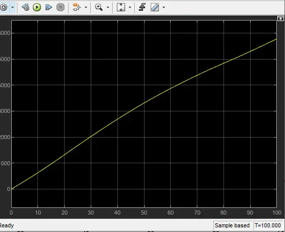
A plot for work done at each instance is displayed below for d = 100 mm.

Part 2-

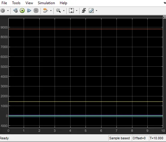
Part 3 –

A mass Spring Damper System-

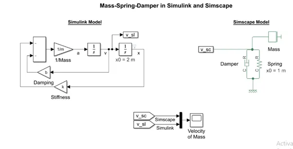
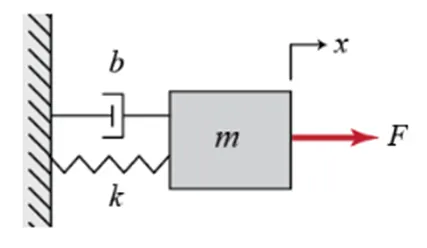
A mass spring damper system is the discretised model of any system.

This system is lumped into a single point mass in the MSD system. the inertial effect of this dynamic system is related to this lumped mass. The stored energy/ the inertial energy of the dynamic system is modelled as a 1-Dimensional spring in the MSD system. the spring is able to store the energy inside when it is stretched or compressed from its original length. The energy dissipated out of the dynamic system is modelled through a 1 Dimensional damper in the MSD system. the viscous damper for instance, is able to dissipate energy as heat outside the dynamic system.

A mass (m) is connected with linear damper (b) and linear spring (k).

Mass Force (F) moves in a positive direction (x).

Spring (K) is an extension, resists the motion of the mass Spring Force (FK) which is again in the negative direction and hence it is negative.

Sum of all the forces we get the equation as –

From the Figure considering the free body diagram, Mass Spring Damper Equation is

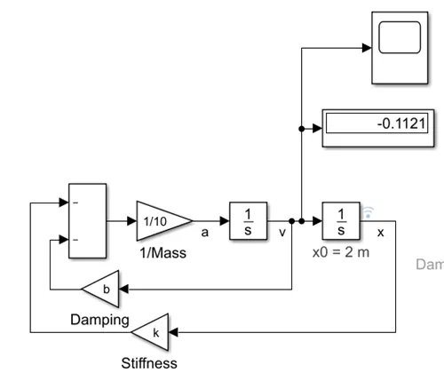
Governing equation of Spring- Mass- Damper

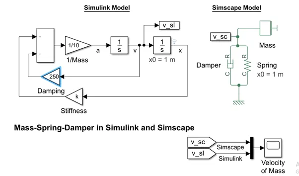
Now we will change the value of Mass, Damper, Spring for the simscape model & plot the results

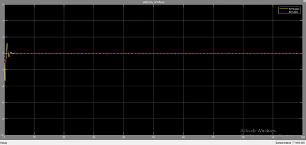
For b = 30 N (M/s), K = 250 N/m, m = 10 kg

Plot-

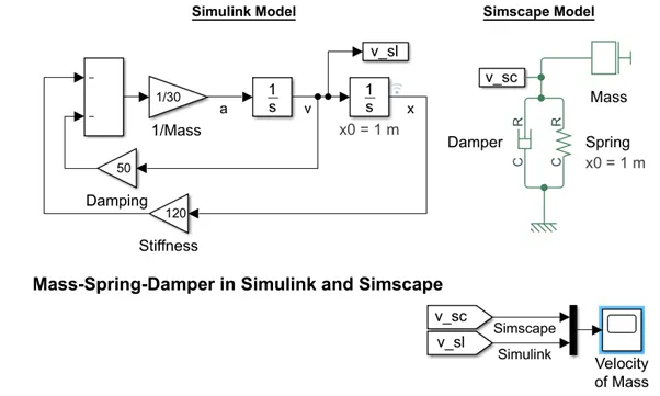
For b = 50 N (M/s), K = 120 N/m, m = 30 kg

Plot-

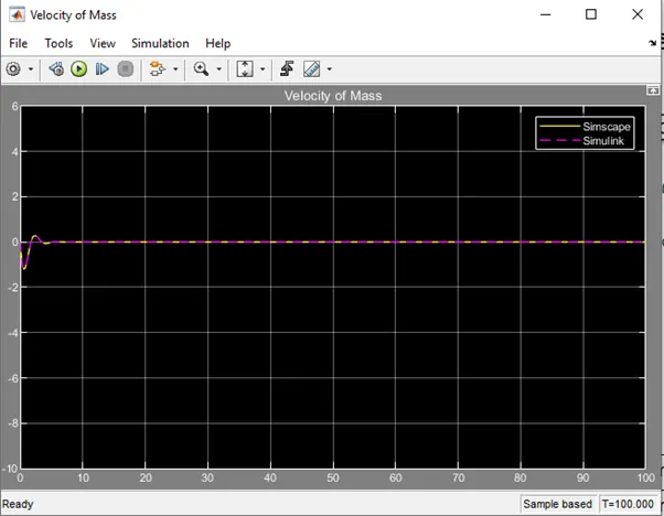
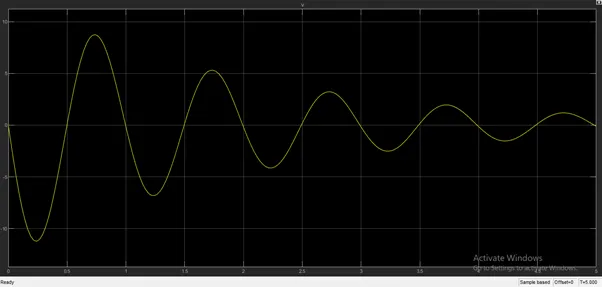
Change the value of mass X₀ = 2 and plot the results & Make the response of Simscape & Simulink as 2 separate displays-

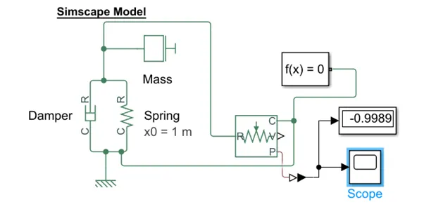
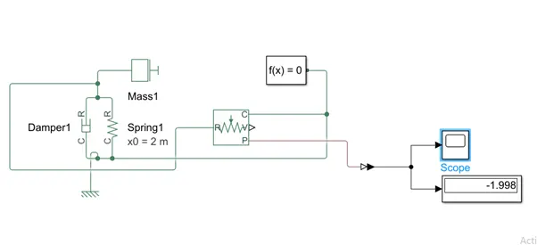
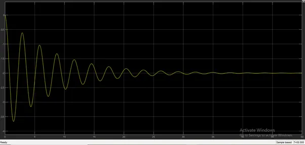
Simscape output –

b = 15 N (m/s)

K = 280 N/m.

m = 60 Kg.

X₀ = 2 m.

Plot-

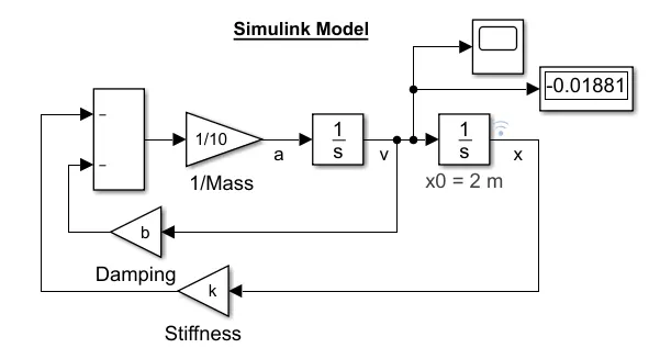
Simulink output –

b = 10 N (m/s)

K = 400 N/m.

m = 10 Kg.

X₀ = 2 m.

Plot-

Study 1 -

Signal Builder is connected with integrator to make integral of distance with respect to time (known as displacement) & it gives the total area between the path & the boundary from the path. Finally, net workdone has also calculated.

Study 2 –

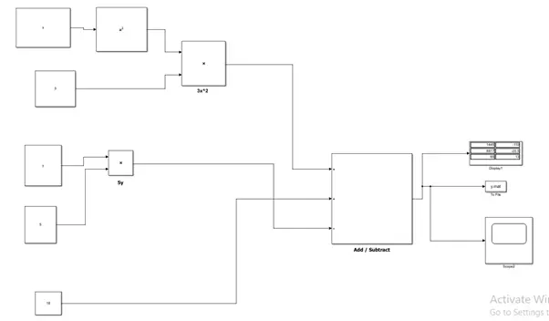
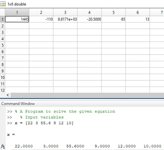
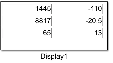
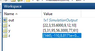
Input values of x& y are taken from MATLAB which already assigned variables and solving the equation Finally z value is displayed in the Display Block & also same z values displayed in the workspace.

Study 3 –

Governing equation of the Mass Spring Damper System Derived by changing the input values of mass, spring, damper for the Simscape Model & Simulink Model & obtained this by increasing the damping value, it will reduce the oscillation of the mass & increasing the spring constant which causes increase in oscillation of the mass. Damping coefficient is inversely proportional to spring constant.

Conclusions-

1. Net workdone is the area under the curve (Force vs. Distance) and found to be 5780 KN.mm i.e. 5780 N.m.
2. All values are displayed in the workspace and stored in the format of y.mat.
3. Governing erquation can be derived into two ways –
   1. Increasing the damping coefficient value decreases the amplitude of the output, incrementing the initial conditions increases the oscillations.
   2. Simulink & Simscape outputs are same irrespective