ELECTRIC RICKSHAW MODELLING

PROJECT – ELECTRIC RICKSHAW MODELLING

Aim –

1. To model an electric rickshaw (Three Wheeled Passenger Vehicle) using MATLAB/Simulink.
2. To drive the vehicle using permanent magnet brushed type motor.
3. To check the efficiency of the system.
4. To check energy consumption and temperature rise of motor and controller for (HWFET, EUDC, Artemis Motorway 130 kmph) drive cycle.
5. To create a custom drive cycle using an excel sheet.

Software Used –

MATLAB R2020a (Simulink).

Introduction -

E – Rickshaw development started in the global market sometime during World War Period, but faded away with time. These were later introduced in China by local and Japanese motor vehicle industries & then further spreaded in areas of Asia. Indian development of e-rickshaw started in late 1990s with the aim of improving manual rickshaws. E-Rickshaw was developed with motor assisted pedal rickshaw (MAPRA) by Nimbkar Agricultural Research Institute (NARI). ELECSHA (Electric Rickshaw) 2000 was also developed later on, but there were issues with battery performance 7 quality due to which these could not trend in market. Illustration of these 2 models given in 2 images below –

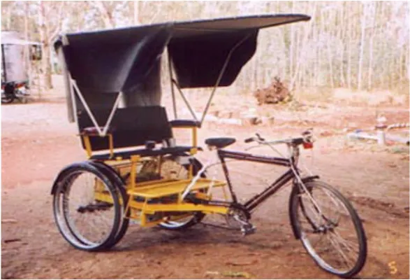
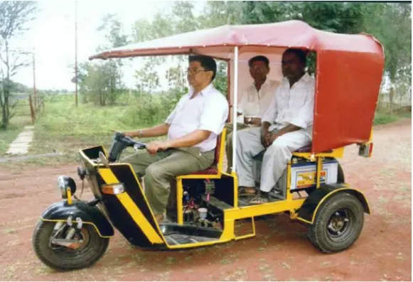
In 1999, Mahindra launched its first electric 3 wheeler & around 2010, E-Rickshaws gained prominence in various urban and semi-urban areas of UP, Bihar, West Bengal & cities of some other states. Delhi NCR also witnessed rise in number of E-Rickshaws during Commonwealth Games 2010. E-Rickshaws were launched in Delhi with the objective to eventually phase out conventional cycle rickshaws, this objective was eventually altered when E-Rickshaws were excluded from NMT category & included in Motor Vehicles Act (2014) as last mile connectivity model option.

As per Motor Vehicles Act 2014 & Motor Vehicles (Amendment), E-Rickshaws were defined as, “A special purpose battery operated vehicles having 3 wheels & intended to provide last mile connectivity for transport of passengers for hire or reward, provided such vehicle is constructed or adapted to carry not more than 4 passengers excluding driver & not more than 40 KG luggage in total; net power of its motor is not more than 4000 W & maximum speed of the vehicle is not more than 25 Kmph.”

E-Rickshaws are latest entry in the Indian Road & Transport System. a flexible, non-polluting & affordable system, they have been playing significant role in solving the last mile connectivity issue. Due to absence of rules and norms, they have been largely operating very informally. While the licencing of E-Rickshaws has been given the nod by the Ministry of Road Transport & Highways, the operation of this system is still ambiguous which has currently led to a ban order by Delhi High Court. Because of the existence of the issue of monitoring and framing rule book for E-Rickshaws for the safety and security of commuters using these systems. Policy Guidelines are required whether E-Rickshaws Are Intermediate Para-Transmit (IPT) system, who is responsible for licencing and regulation & how it gets integrated 7 act as a feeder to the public transport. Specific provisions are required to address the question on speed, vehicle specification s and insurance, lane traffic and fare charges & this requires policy framework to address the concerns of both the E-Rickshaw drivers and its counterparts.

Centre of Public Policy Research (CPPR) believes that E-Rickshaw needs to be integrated into the system at the policy as well as the infrastructure level & developed as an appropriate feeder system. this demands for a need bases assessment and defining of IPT characteristics in the current public transport system of India. This policy briefly aims to develop an approach wherein the systems like E- Rickshaw shall be formally integrated and devised to support the existing system & enable a sustained transport system.

Advantages of E-Rickshaw –

1. Solving Last-Mile issue.
2. Green Mode of Transport.
3. Ease of Access.
4. Easy procurement process.

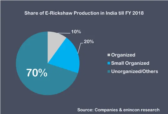
Electric Rickshaws have been widely accepted as alternative Petrol/Diesel/CNG auto rickshaws. They are wheelers pulled by an electric motor ranging from 650-1400 Watts & mostly manufactured in India & China, only few other countries manufacture these vehicles.

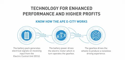
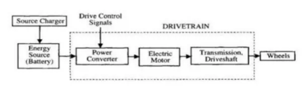
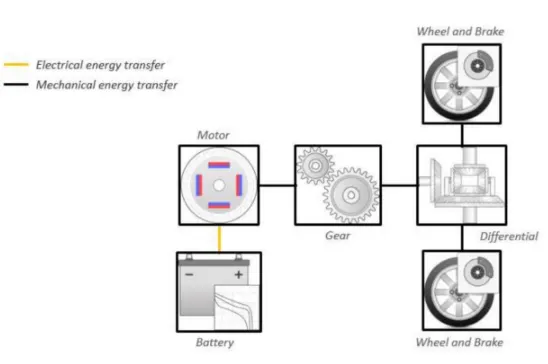
Electric Rickshaws are very simple to operate than ICE rickshaws and the simplest powertrain architecture consists in a high voltage battery, an electric motor with power electronics controller and a single speed gearbox. BEVs are also called Pure Electric Vehicles.

In a BEV propulsion is based exclusively on the electric energy stored in the high voltage battery.

Battery electric vehicles are increasing their market share because they are most viable way towards a clean and efficient transport system. compared to ICE vehicles, the most important advantage of a BEV is the overall high efficiency, Reliability & Relatively low cost of the electric motor & the main drawback is the low energy density of the high voltage battery.

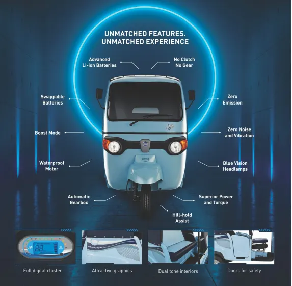
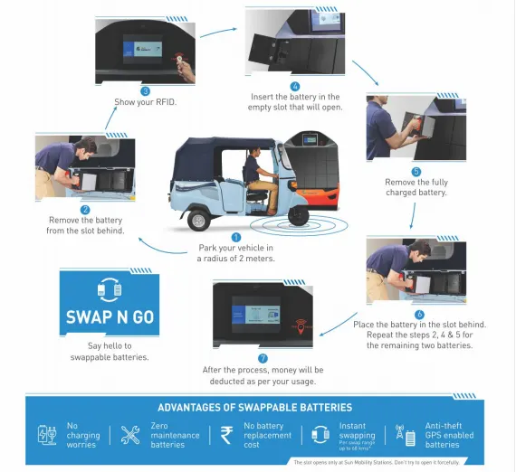
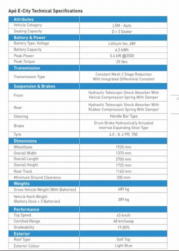
Let us consider Appe E-City Piaggio.

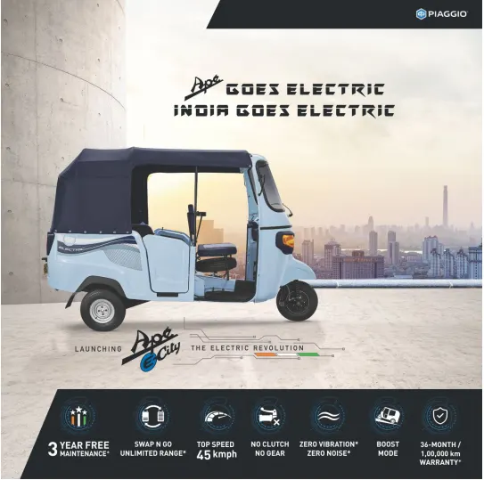
Block Diagram of E-Rickshaw –

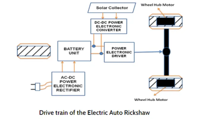
Drivetrain of Ape –e city –

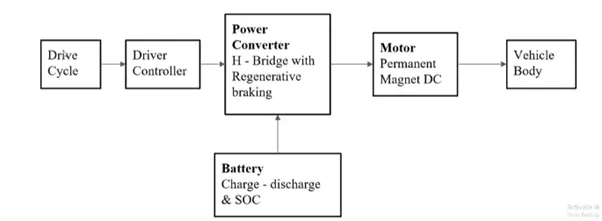
In the designed E-Rickshaw the main blocks are Battery, Drive Cycle, DC Motor, Vehicle Body and Transmission System. drive cycle is the input data like a how a human drive his actual vehicle here FTP75, WOT, Excel (Manually prepared in excel sheet) drive cycles are used to make the designed vehicle to give the output how it reacts to the drive cycle. The main objective is to obtain the speed by the driver, to estimate the temperature of the motor & controller, to estimate the State of Charge (SoC), Distance travelled by the vehicle. There is a SOC block that will estimate the State of Charge of a battery, distance is calculated by speed and time parameters for all the drive cycles.

System Level Configuration -

1. Drive Cycle.
2. H- Bridge.
3. DC Motor
4. Battery Source.
5. Controlled PWM Voltage.
6. Vehicle & others.

Model Parameters –

Drive Cycle –

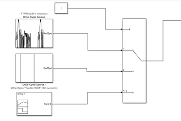
Drive cycle is assumed as the driver’s input of the vehicle, it replaced how a driver will drive a vehicle. Here I have used 3 drive cycles which is used to test vehicle performances. These drive cycles will have high speed, low speed braking conditions in it. There are different drive cycles like WOT, FTP75, etc. here is the model I have used FTP 75, WOT & Drive Source which is manually prepared in excel.

Manually Prepared Drive Cycle –

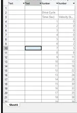
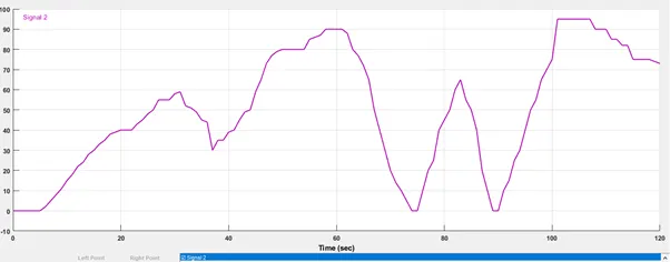
Link – https://drive.google.com/file/d/1j-nolR8h_Mc1udrqosvvZfeXizU8LsgM/view?usp=sharing

FTP 75 –

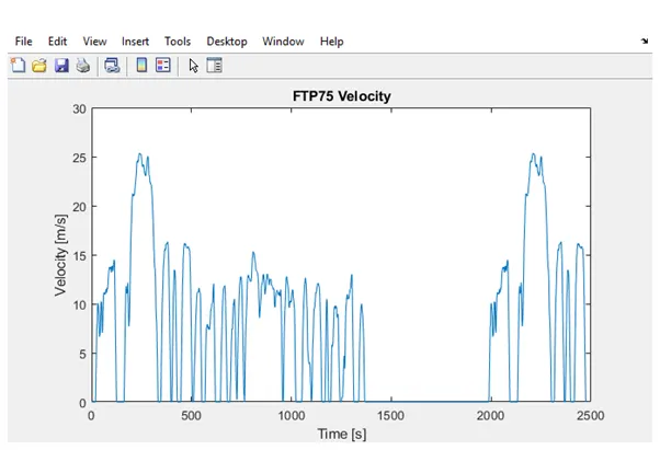
Generated a standard or user specified longitudinal drive cycle. The block output is the vehicle longitudinal speed. You can import drive cycles from:

• Pre-Defined Sources.
• Workspace variables including arrays & time series objects.
• mat, xls, xlsx, or txt files.

Use the fault tracking parameters to identify drive cycle faults within specified speed and time tolerances.

Wide Open Throttle (WOT) –

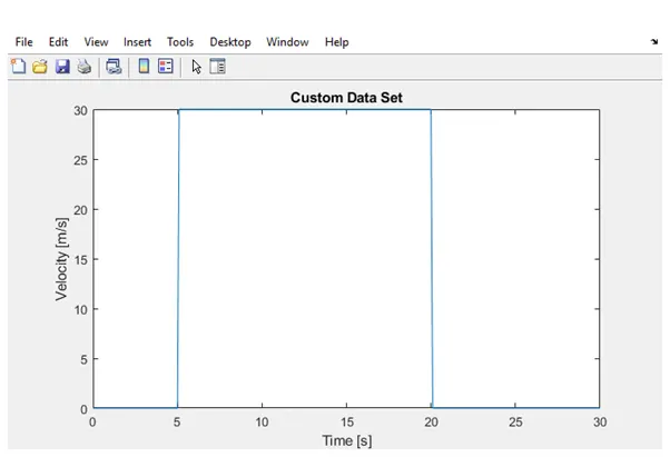
All 3 drive cycles are controlled by the controller provided above by constant through Multi-Port Switch.

Drive Controller –

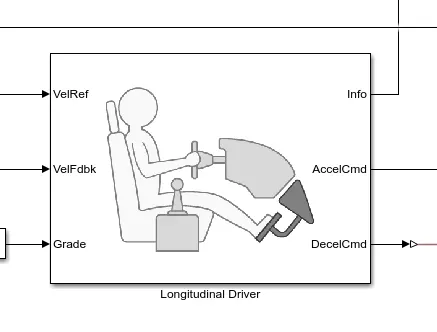
A parametric longitudinal speed tracking controller for generating normalized acceleration & braking commands based on reference & feedback velocities.

Use the external actions to input signals that can disable, hold or override the closed loop commands determined by the block. The block uses this priority for the input commands: Disable, Hold, Override.

Drive cycle is connected to a longitudinal driver, it has 6 ports namely velocity reference, velocity feedback, Grade, Info, Acceleration, Deceleration.

VelRef is given by the Drive cycle data & VelFdbk is given by the output of the motor. These 2 will get compare & the acceleration or deceleration output will be given to the motor controller. Accelcmd is given the PWM generator block and deccelcmd is given to the regenerative port of the H-Bridge which uses to generate regenerative braking. Info is used to get any other data from a longitudinal drive block. The grade is to give the input of gradebility to the driver block. This block helps to generate the driver’s conditions of the vehicle using the drive cycle block. Here default parameters & controlled type PI is used.

Motor & Controller -

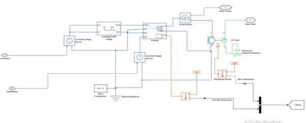
1. Motor Type: DC Motor (PM Brushed Type Motor) –

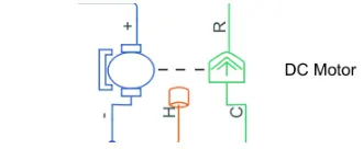
This block represents electrical & torque characteristics of a DC motor includes thermal port to sense the temp. of the motor.

The block assumes that the no electrical energy is lost & hence the back-emf & torque constants have the same numerical value when in SI units. Motor parameters can either be specified directly or derived from no load speed & stall torque. If no information is available on armature inductance, this parameter can be set to some small non-zero value.

When a positive current flow from the electrical + to – ports, a positive torque acts from the mechanical C to R ports. Motor torque direction can be changed by altering the sign of the back-emf or torque constants.

Motor parameters –

Armature Inductance - 12e-6

No-Load Speed - 3000 RPM.

Rated Speed – 1500 RPM.

Rated Load – 1 Kw.

Rated DC Supply Voltage – 48 V.

Rotor Inertia – 0.01

Thermal Mass – 20 kJ/K

Initial Temperature – 25 Degree Celsius.

The Motor Controller will get input from the longitudinal driver. Its tasks are to control the speed of the motor and drive according to the input of the driver. Motor Controller generally has 2 main parts mainly PWM Voltage generator & H-Bridge.

Input1 is getting from the Accelcmd of a longitudinal driver & it is given to a controlled voltage source block where it is input to the controlled PWM voltage & will generate the PWM Signal in such a way that H-Bridge will generate the required voltage to operate the DC motor for the given driver input. PWM voltage block negative reference & REF are grounded & REF of H-Bridge respectively. H-Bridge is a motor controller that has IGBT components aligned in the shape of H & will operate only 2 at a time respectively to the i/p of the signal from the PWM block. When deceleration occur this H-Bridge will give an output from the positive & negative terminals of it. These positive and negative terminals are connected to the DC motor & battery. All these components are the Simscape electrical components so they need a connection to the solver configuration block which helps to solve the Simulation.

Controlled PWM Voltage Source –

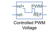
This block creates Pulse Width Modulated (PWM) voltage across the PWM & REF port. The output voltage is zero when the pulse is low & is equal to the output voltage amplitude parameter when high. Duty Cycle is set by the input value. Right-Click the block & select Simscape -> Block choices to switch between electrical +ref/-ref ports and the PS input u to specify the input value.

At time zero, the pulse is initialized as high unless the duty cycle is set to 0 or the pulse delay to time is greater than zero.

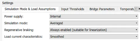
The simulation mode can be set to PWM or Averaged. In PWM mode, the output is a PWM signal. In averaged mode, the output is constant with value equal to the averaged PWM signal.

Select simulation mode as Averaged.

Power Converter (H-Bridge) –

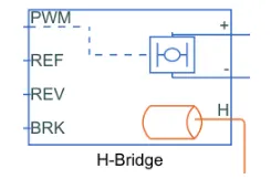
H-Bridge is used as a DC-DC Converter –

This block represents the H-Bridge motor drive. The block can be driven by the controlled PWM voltage block in PWM or Averaged mode. In PWM mode, the motor is powered if the PWM port voltage is above the Enable Threshold Voltage. In Averaged mode, the PWM port voltage divided by the PWM signal amplitude parameter defines the ratio of the on-time to the PWM period. Using this ratio and assumptions about the load, the block applies an average voltage to the load that achieves the correct average load current. The simulation mode parameter value must be the same for the controlled PWM voltage & H-Bridge Blocks.

If the REV port voltage is greater than the Reverse Threshold Voltage, then the output voltage polarity is reversed. If the BRK port voltage is greater than the braking threshold voltage. Then the output terminals are short circuited via one bridge arm in series with the parallel combination of a second bridge arm & a freewheeling diode. Voltages at port PWM, REV & BRK are defined relative to the REF port.

If exposing the power supply connections, the block only supports PWM mode.

Motor Controlled Parameters –

Threshold Voltage – 2.5 V.

PWM Amplitude – 5 V.

Reverse Threshold – 2.5 V.

Braking Voltage – 2.5 V.

Output Voltage – 200 V.

Temperature Sensor –

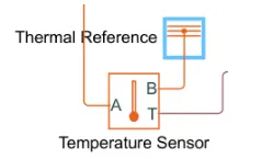
Temperature sensor is used to measure the temperature of H-Bridge & Motor.

This block measures temperature in a thermal network. There is no heat flow through the sensor. The physical signal port T reports the temperature difference across the sensor. The measurement is positive when the temperature at port A is greater than the temperature at port B.

Solver Configuration –

Defines solver settings to use for simulation.

References –

Electrical Reference – Used to ground all the electrical components.

Mechanical Rotational Reference – Used to ground all the mechanical rotational parts.

Thermal Reference – Used to ground the Thermal Sensor.

Lithium-Ion Battery –

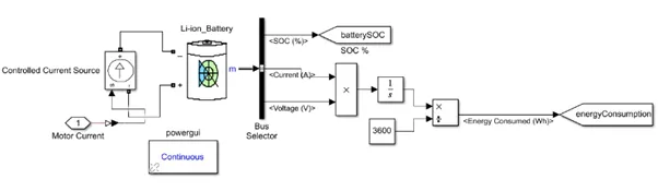
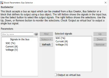
Battery Type – Lithium Ion.

Nominal Voltage – 330V.

Rated Capacity – 75Ah

Initial SoC% - 100

Internal Resistance – 0.0012 Ohm.

The battery is required to power the controller and the motor. The controller uses the battery power according to produce the input given by the motor to obtain maximum speed. The battery is also used to power to produce the input given by the motor to obtain maximum speed & also used to power every electrical component in the vehicle. The battery has 2 stages one is charging and another one is discharging state. The battery is of 75Ah capacity.

The nominal voltage of the battery is 330V.

Initial SoC % is of 100%.

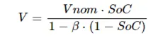
The battery as a series internal resistance plus a charge dependent voltage source defined by:

Where SoC is a State of Charge and V_nom is the nominal voltage. Coefficient beta is calculated to satisfy a user defined data point [AH1, V1].

The battery has a positive and a negative terminal which is given the voltage controlled source where the battery consumption is controlled by the motor controller and then it is given to the SoC block.

State of Charge (SoC) –

SoC is the percentage or level of the battery presents after certain level or consumption of battery charge by the vehicle. Battery charge or SoC is calculated by the giving it to the rate transition & then to gain where 1/(Nominal Battery Capacity) then to a discrete time integrator & it will get minus from the 1 as it is considered 100% of battery & it is multiplied with 100 to get percentage of battery.

The majority of blocks are Simscape blocks where Physical to Simulink Converter is used to convert the physical signal from Simscape block to Simulink Signal.

The circuit parameters can be modified to represent the specific battery type & its discharge characteristics. A typical discharge curve consists of 3 sections –

A basic block configuration & steps involve during the whole system analysis -

• Blocks used –
• Power GUI.
• Controlled Current Source.
• Battery.
• Temperature Ambient.
• Bus Selector.
• Integrator.
• Divide.
• Product.
• Time.
• Scope.

Vehicle Body & Transmission –

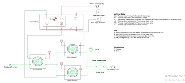
Motor will produce the rotational output which will give to the vehicle body & transmission system. the rotational output is taken by the gear system here to maintain the constant speed throughout the transmission without any loss in speed from the motor to tires.

The gear output is given to axles of rear tires, in the circuit it is shown that gear is connected to rear wheels & front tire is free to rotational motion, thus vehicle moves forward. N is the normal force caused by the tires & it is given to the vehicle body normal force port. The vehicle body has an H-hub, S –Tire Slip, N –Normal Force, A –Axle Connection, wind velocity, inclination angle. The tire hub is connected as a common node to the vehicle body. The vehicle body wind velocity is connected to a constant block & the beta-inclination angle is connected to another constant block where we can assign wind velocity & inclination angle as per requirement. Velocity is the output port where we can get at which speed the vehicle is moving. The velocity is taken out to get the distance travelled & State of Charge.

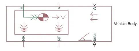
The above figure highlights the vehicle body for electric rickshaw which is having rear axle drive. The vehicle body block represents a 2 axle vehicle body in a longitudinal motion.

The block consists body mass, aerodynamic drag, road decline & weight distribution among axles due to acceleration and road profile (optionally we can include Pitch & Suspension Dynamics).

In a given block –

NR – Physical Signal Output which is connected to the rear wheel axle. For this model, it is connected with a normal force of rear tire.

NF – It is Physical Signal output which is connected to front wheel axle & for this particular model it is connected with normal force acting on a front wheel tire.

Beta – Beta is basically a road incline angle.

V – This port is Vehicle’s longitudinal velocity.

W – it is the headwind speed. Basically, we will define a particular wind speed by adding constant block.

Parameters of Vehicle body

Mass – 615 kg.

No. of wheels per axle – 2

Frontal Area – 1.48 m²

Drag Coefficient – 0.5

Air Density – 1.18 Kg/m³

Wheels Modelling –

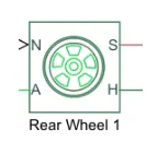
The tire (Magic Formula) block models a tire with longitudinal behaviour given by the magic formula, an empirical equation based on four fitting coefficients. The block can model tire dynamics under constant or variable pavement conditions.

The tire (Magic Formula) block models the tire as a rigid wheel tire combination in contact with the road and subject to slip. When torque is applied to wheel axle, the tire pushes on the ground (While Subject to contact friction) & transfers the resulting reaction as a force block on the wheel. The action pushes the wheel forward or backwords. If you include the optional tire compliance, the tire flexibility deforms under load.

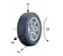
The figure shows forces acting on the tire -

Where,

Fx – Longitudinal force exerted on the tire at the contact point.

Fz – Vertical load on the tire.

Omega – Wheel angular Velocity.

Vx – Vehicle hub longitudinal velocity.

In the particular block -

N – Normal force acting on tire & connected with NR of the vehicle body.

S – Slip between the tire and road connected with Goto block.

H – Hub and it is used to find the thrust created by the tire & it is connected with H input of vehicle body also including all four Hub of the wheel.

A – Axle and rear axle are connected with the (Simple gear) final drive system & the front axle is connected with the left & right wheel.

Parameters of Wheels –

Wheel Radius – 0.306 m.

Vertical Load – 3000 N.

Peak longitudinal force at rated load – 3500 N.

Slip – 10.

3. Inertia –

Inertia – 0.01 Kgm²

The block represents an ideal mechanical rotational; inertia.

The block has one mechanical rotational conserving port. The block positive direction is from its port to the reference point. This means that the inertia torque is positive if the inertia is accelerated in the positive direction.

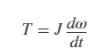
4. Simple Gear Box –

Gear ratio represents a fixed-ratio gear or gear box. No inertia or compliance is modelled in this block. But there is an option to include gear meshing & viscous bearing losses.

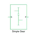
Connections B (base) & F (Follower) are mechanical rotational conserving ports. Specify the relation between base & follower rotational direction with output shaft rotates parameter. Optionally include thermal effects & expose thermal conserving ports H by right click on the block and selecting Simscape block choices to switch between variants.

Output shaft rotates in the same direction of the input shaft.

Base is connected to the motor shaft & the follower is connected with the rear wheel drive.

PowerGUI –

The PowerGUI block allows us to choose one of these methods to solve your circuit –

• Continuous, which uses variable step-solver from Simulink.
• Discretization of the electrical system for a solution at fixed time steps.
• Continuous or discrete phasor solution.
• The PowerGUI block also opens tools for Steady-State & Simulation results analysis & for advanced parameter design.
• For calculating the SoC (State of Charge) we have to create a subsystem which will consist of Rate transition, Gain, Discrete Time Integrator, Constant & Sum blocks.

Plots –

Results –

1. For FTP 75 Drive Cycle –

By running the vehicle with FTP 75 Drive cycle for 2474 Sec. the distance travelled is 19.44 Km.

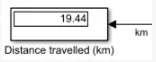
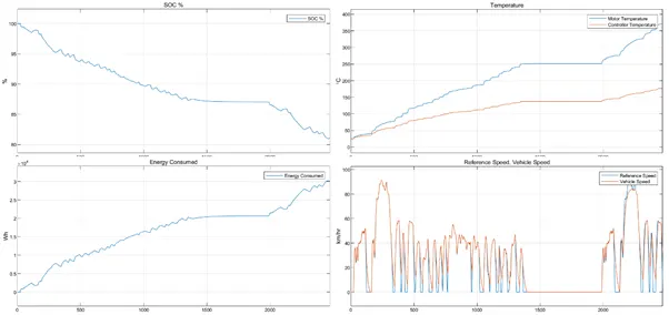
• The actual speed is approximately followed the 90% of reference drive cycle.
• Energy consumed by the battery is approximately equal to 3.10⁴ Wh at the end of drive cycle.
• The SoC % of the battery is reduced to nearly 83%.
• The temp. of the motor is increased to 370 Degree Celsius.
• The temp. of the controller is 180 Degree Celsius.

For WOT Drive Cycle –

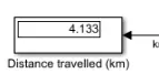
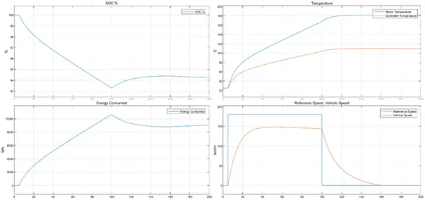
• The actual speed is approximately followed the 85% of reference drive cycle.
• Energy consumed by the battery is increased linearly till 100 sec. to approx. 1050 Wh and then reduced gradually due to back emf & finally at the end of the cycle the energy consumption is reached to 900 Wh.
• The SoC % of the battery is reduced to 91% at 100^th after that 100 to 200 Sec. the battery get charged by back EMF. Finally, at the end of the 400^th second the SoC is approx. equals to 94.2 %.
• The temp. of the motor increased to 180 Degree Celsius.
• The temp. of the controller is 110 Degree Celsius.

For Manually Prepared Drive Cycle –

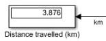
To increase the speed of the vehicle the output voltage amplitude is applied to 400 V.

By running the vehicle with manually prepared drive cycle for 120 Sec. the distance travelled is 3.87 Km.

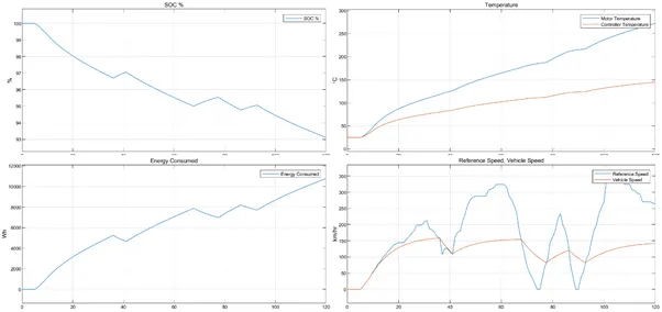
The actual path of the speed is approximately followed the reference drive cycle as above.

Energy consumed by the battery is varied with respect to time & distance nearly equal to 10500 Wh at the end of the cycle.

The SoC% of the battery is reduced to 94.2 %.

the temp. of the motor is increased to 260 Degree Celsius.

The temp. of the controller is 145 Degree Celsius.

Conclusion –

1. Here there is a compromise with the temperature of the motor & controller to achieve vehicle speed which is near to reference speed. Since I haven’t used any cooling system in the model. In the real time application, the motor temperature is less than 100 degrees Celsius.
2. In the Real time application, the motor, battery & controller temperature is controlled by air cooling. Hence, the temperature of this components is not increased to this extent.
3. Created a MATLAB model of an electric rickshaw (3 Wheeled Passenger Vehicle) by using Li-Ion battery. PM brushed type DC motor.
4. Determined the variables of temperature of motor & controller, SoC% & Energy consumed by the vehicle for all the 3 reference drive cycles (i.e. FTP75, WOT, Manually Prepared).
5. This battery powered rickshaw will be most popular mode of transport in future.

EV Rickshaw Model - https://drive.google.com/file/d/1fg1ZmykDeHPSuQPKwHTzz0sQjs_I_fxA/view?usp=sharing