Week 5 Challenge: Analog Control Systems

1. Compare analog control system with digital one with respect to electric vehicle motor.
2. Explain call back and over the air update events by automotive companies.
3. Using MATLAB plot bode diagram of chosen transfer function in s-domain and z-domain. Comment on the results.

1. Compare analog control system with digital one with respect to electric vehicle motor.

The word ‘digital’ and ‘analog’ preceding ‘control systems’ do have their literal meaning in electronics.

Analog control system deals, processes and outputs continuous values between a certain range (theoretically infinite, but practically all actuators are limited to a certain range) while digital makes use of an intermediary binary language for all sorts of computation before it is converted back to analog using digital to analog converters.

Since manipulating a continuous signal is much harder, and with advent of powerful computers in recent years, most of control system are digital just because they’re just a whole lot easier to deal with in so many circumstances with the only real addition being ADC and DAC in the process pipeline between the input and output states.

Advantages of digital are as follows

1. Digital signals are very resistant to noise since most communication in the pipeline is usually done in 1s and 0s. Noise interference with these signals hardly causes any distortion in the original signal. And moreover noise filters during the computation process can usually take care of any noise, if induced
2. Since analog signals needs to inevitably be quantized to digital signals (quantized, meaning the continuous signal needs to be discretized into small steps), the resolution of the signal is significantly reduced. However, an upside to this is that this reduces a great deal of load for computation and storage purposes. And these days, computers have become powerful enough to process a signal with extremely small discretization steps, thereby mostly overcoming the aforementioned resolution loss.
3. As a direct result to above point, power efficiency is also dramatically increased
4. Devices that usually process purely in analog tend to degrade or get damaged over time and needs to be constantly checked, or calibrated while in digital control systems, only the input sensor device and actuators usually have to be calibrated, making maintenance much easier

General Difference between Analog & Digital Control

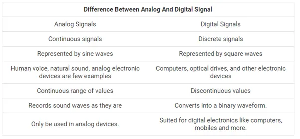
General Difference between Analog & Digital Control

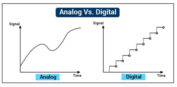
Difference between Analog & Signal Waveform

Faster and cheaper processors currently being turned out by the silicon foundries are making it easier to justify digital drives instead of traditional analog drives. But do digital drives offer a clear advantage for more applications?

Compare the two approaches by first analyzing the classic analog drive shown in the diagram. In this case, the drive is configured as a torque amplifier. An external controller generates a ±10-Vdc command signal. The drive monitors the motor winding current and estimates the mechanical torque. A compensator takes the difference and generates a voltage command signal. Next, a pulse-width-modulated signal is applied to an inverter, which switches the correct voltages to the motor.

Contrast this to the equivalent digital drive system as illustrated. Most of the analog circuitry (summing amplifier, scaling amplifier, compensator, and PWM generator) is hidden in the large block called calculations, while the power inverter is identical. Because the calculations are all done in software, different concepts, such as new compensation-scheme algorithms, can be programmed on the fly and evaluated much faster than with an analog system (minutes instead of hours). This helps drive companies develop new, advanced features more quickly.

From a user's perspective, the main difference is in how the signals are obtained. Both the current and torque signals need to be converted to digital representations. This is done by a sample and hold (S/H) circuit and an analog-to-digital converter (ADC). The sample and hold circuit takes the value of the analog signal at a specific instant in time and freezes it. The frequency at which this is done is known as the sampling rate, for example, 4 kHz. The frozen signal is then converted into a digital value with a specific number of bits. The more bits that are used, the more accurate the digital representation. For example, a 12-bit converter provides approximately 5 mV of resolution on the torque command. This quantization effect needs to be considered when selecting a drive.

One of the main advantages of a digital drive system is the ease with which new features can be added. If it has sufficient processing power, additional functions can be added for only the cost of development. For example, consider the active damping feature first introduced on steppers. The analog drive circuitry required more than 100 components. Obviously, this had to be accounted for early in the design. When the active damping feature was implemented in the digital drive, it merely consisted of several lines of code. With sufficient processing power, features such as encoderless stall detection, which would be nearly impossible to do in analog, can be economically added to the drive.

Another advantage of a digital drive is the ease with which it is field upgradable. Using flash memory, new software can be posted on a Web site or e-mailed to customers. This lets new features and bug fixes be easily delivered to the field without sending the drive back to the factory. Custom software specifically tailored to a single customer's application is also possible.

Digital systems do have some shortcomings relative to analog ones, however. One major issue concerns the sampling delay. The controller sends out a torque command, but by the time the drive control algorithm receives the digital value, several hundred microseconds have passed. This sampling delay can reduce the overall bandwidth of a motion system. The sampling delay in the torque command also affects the current feedback. Digital systems use pulse-by-pulse current control, while the current is continuously monitored in an analog compensator. When the current reaches the maximum threshold, the voltage immediately shuts off. The duty cycle for a digital system is invariant and could allow the current to exceed the maximum value as shown in the figure. This can be a significant problem in low inductance systems where large current ripple exists and the rate of current change is approximately the bus voltage divided by the inductance.

Although analog drives are typically less expensive than digital ones, the controller often is integrated into the digital drive, which can reduce overall system cost. Analog drives are also easier to set up, with DIP switches being set rather than having to program the parameters so initial motion profiles can be generated quickly. However, digital drives offer more parameter variations, which lets system designers have more options.

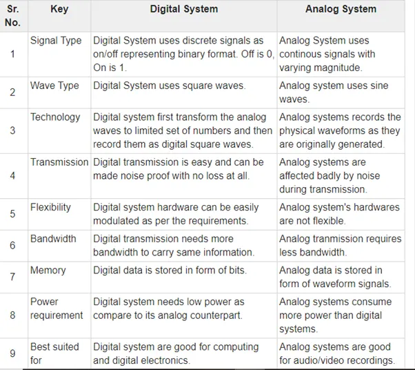
Comparison on basis of selection criterion

2. Explain call backand over the air update events by automotive companies.

Now-a-days EVs & HEVs Call-Back function isn’t much used instead of that ‘Over the Air (OTA)’ is used. Call-Back events used in Automobile industry to call back or recall the past history if they face any problem or difficulty or fault while manufacturing the vehicle.

Whereas, OTA is a new adopted process where the companies need not to call-back or go or visit the garage or factories and solve the problem without any difficulties. before, Call-back used in previous days. This was done when a vehicle had fault in it. Then the car manufacturer will just call back the previous cars so that they can rectify the fault in it and make the required improvements.

Vehicle is a dynamic system and it is required to tune the system. there are 2 ways to tune 1) By Tools 2) By Fundamentals. Direct tuning doesn’t help always in such cases with the help of real-time tuning we can tune it accordingly with the help of microprocessors.

OTA is a new adopted approach where the companies need not to call back, go and visit the garage or factories & rectify the faults and follow required procedures without other cumbersome processes.

Updating software and firmware using Over-the-Air (OTA) has increased in the handheld devices, industrial, and automotive sectors for the embedded platform with time. Once the product is in the real world, firmware or the software update related to bug fixes, security fixes, or the feature update is required for the betterment of the device and keeping it updated with latest software.

OTA is a technology to update the software or the firmware remotely.

In case of a vehicle, the firmware or software is updated wirelessly using a telecommunication device, through a gateway inside the car to the ECU whose presence is increasing in modern vehicle.

What is the Need of OTA (Over-the-Air Update) for the Vehicle?

In Automotive industry, the vehicle has become more and more intelligent and smart. Currently, the vehicles are majorly controlled by a software rather than traditional mechanical components.

A decade ago, if there was a need to update the software the vehicle was towed to the service station and the vehicles were connected to the system/computer for an update. OTA solves the problem of reliability of each updated that used to be present earlier, secondly dependency of the service station, carrying the vehicle to the station, the cost of update the software becomes very low, and no much hassle to the customer and well as the service station. Last but not least, the security update on time for every vehicle is important and is done at easeThe approach of the OTA update for the mobile phones and the vehicles are different, the vehicle OTA update is more complex and stringent as compared to the handheld device, improper software update may cause harm to user life too.

Electronic Control Units (ECUs) has become the major component in the vehicle today, ECU has replaced all mechanical steering components. In general, ECUs are interconnected by one or more networks and share information that enables complex interactions and regulations. For example, In Advanced Driver Assistance Systems (ADAS), the increasing functional capabilities comes with a higher system complexity, which makes software bugs more likely to occur that might have implications for the safety and security of the whole vehicle. With regular software updates and enhancements, one can ensure the systems’ correctness, efficiency, and reliability over the complete lifetime of the vehicle.

This blogs mainly describe the end-to-end solution that can be deployed to support OTA software updates in the automotive sector.

In the previous section, we talked about the OTA and understand that OTA update in the automotive sector has major challenges in terms of security while updating the software over the air.

If the attackers get control of the vehicle, one might end up in a hazard situation.

• Engine transmission can be turned on/off
• Passengers or the drivers can be locked inside the car
• Blowing the horn continuously
• Controlling the steering system
• Car braking system
• Speeding the car beyond road regulation.
• Controlling the navigation, audio or infotainment system
• False alarm in the cockpit

Let’s see how the OTA update happens in the vehicle.

Overview: The OTA remote update method of the vehicles is fast, cost-effective, and allows updating of the software running on their ECUs over-the-air, and the car users can update the software anywhere without having to go to the service centre or repair shop. Further, OEM can diagnose the car based on the data received through over-the-air from the car.

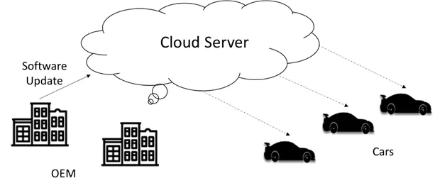
Secure OTA in the automotive system: The secure OTA update is the most important factor while updating the firmware or software for the ECU. There are a lot of challenges to achieve secure OTA update. There are many techniques proposed and implemented across the industry to achieve the secure OTA updates. We will be discussing some of them and explain the most common technique used in the automotive industry.

Let’s divide the whole end-to-end architecture into three components and what is the purpose of it.

Backend Server

• Create the updated images/Collect the images from the different Tier-1
• Provide the firmware and software update images to flash to the device
• It might need to support client-server architecture, if the head unit request for the update.

Communication Channel

• Provide secure mechanism
• Provide the secure n/w so that image or data does not tampered.

Head Unit

• Might need to trigger the software update (client)
• Make sure the correct images are installed
• Less down time while updating the images
• Roll back happens in case of failure

Backend Server: The backend server is mainly responsible for creating the firmware and software images that need to be deployed in-vehicle units. The backend server tries to collect the images that need to be deployed from the different Tier-1 suppliers and packed it in one single image for all the ECU.

This backed server can be based on the Yocto based system (open source) or third-party support architecture.

Communication Channel: The most challenging part of the component is when the data/Images are exposed to the n/w and they are easy for the attackers to manipulate. There are many techniques, open-source and third-party solution for secure update to the head unit

Most commonly used is Uptane. Uptane is the first comprehensive security framework guiding the implementation of OTA update systems on a design level.

Head Unit (Vehicles itself): Head units comprise of many ECU’s, maybe some are high speed, or some less speed, and also different type of ECU, TCU (telematics control unit), gateways, every component as a role to play in the OTA update.

The head unit also needs to make sure that it is ready to connect to the backend to get updated firmware and software. Or itself has the capability to trigger to request update.

OTA update using Uptane

The Update Framework (TUF) is designed to create a security system to protect users of software repositories from the security attacks. It has been designed, keeping in mind that the backend server may not be secure, or the key used for the cryptography can be stolen.

So, what it does is it creates a distributed system, where the dependency on a particular system is not there, and in case of the attacker’s thread, all the systems cannot be hacked so easily at the same time.

The Update Framework (TUF) has divided the roles into four parts (Root of trust, Timestamps, Snapshot, Targets)

Uptane builds on The Update Framework (TUF), which is distributed (Timeserver, directory and image repository, manifests, Primary/secondary ECU’s, full and partial verification.

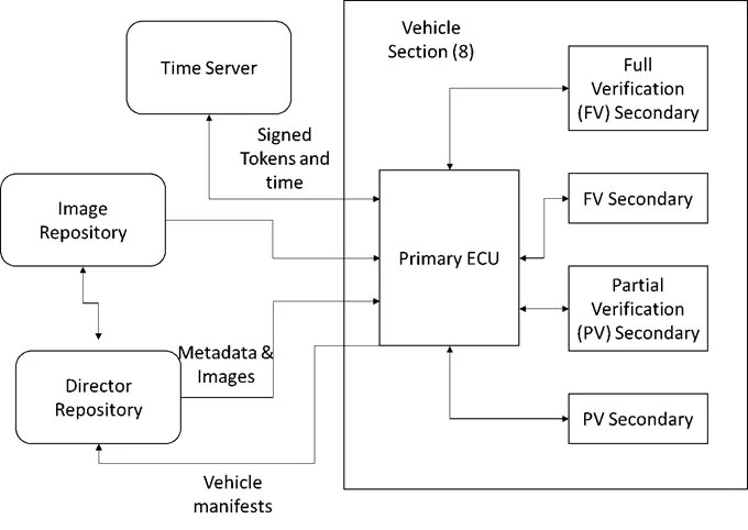
Backend Server:

It will contain the images (the data that need to be updated to the ECU) with metadata (cryptographic hashes, file size)

Image Repository: Image repository uses an offline key to sign the metadata for all available updates for the ECU.

Periodically (e.g., weekly, monthly) update metadata about available images
Use Uptane command-line tools to generate the metadata
Use threshold of offline keys (e.g., Yubikey, HSM, etc. often used) to sign metadata

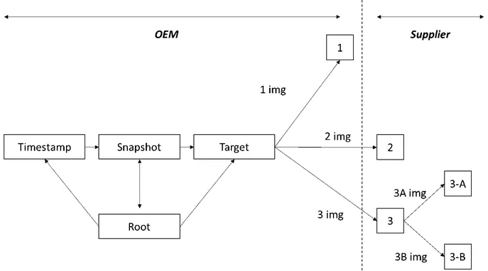
Directory Repository: Directory repository used the online key to sign metadata to be used to install in ECU on the vehicle. It determines which images need to be installed in which ECU’s, create different metadata for the different vehicle, and access the inventory data to get details about the vehicle.

Typically used to instruct a vehicle which updates to install, depending on what it has

• Can be used to instantly blacklist updates
• Use Uptane API to generate signed metadata
• Uses an inventory database to read and write information about ECUs (e.g., public keys, what was previously installed, etc.)

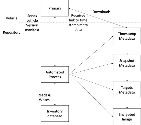
So, the key here is that’s, before installation, it needs to confirm that the instruction from directory and image repository matches.

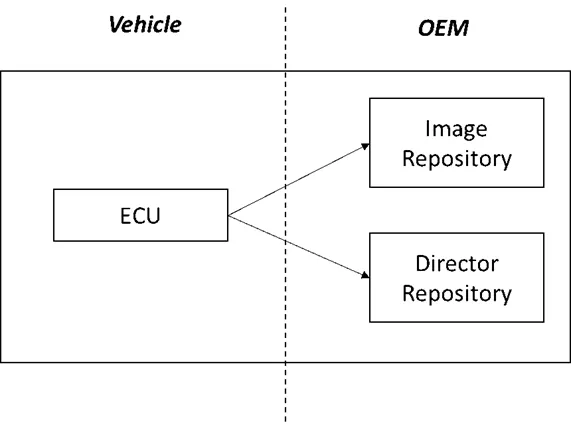
Time server: When the primary ECU sends the list of tokens for every ECUS, to the time server, time server returns a signed message containing the list of tokens and the current time

Head unit (Vehicle Itself):

In the head unit of the vehicle, we have a different type of ECU based on how they connected internally or the external world, how powerful in terms of speed, storage, etc.

• The primary ECU (TCU) download the images, verifies it and then distribute the metadata to the other secondary ECU’s
• The secondary ECU’s also verify the image before updating the images.
• It does the full and partial verification

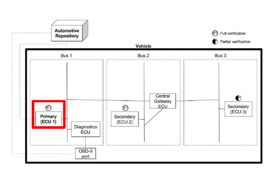
Communication Channel -

Complete flow of communication from the head unit to the Backend server.

• Figure 7: Communication channel
• What does it take to deploy the Uptane?
• The OEM sets up and maintains
  • Director repository
  • Image repository
  • Time server (optional)
• Images are signed by
  • Supplier, or OEM, or Both!
• ECUs shall do either
  • Full verification, or
  • Partial verification
• May keep using your existing TLS, etc. transport
  • If transport / caching compromised, little security risk

Challenges on OTA update

• Automotive is more complex architecture with an increasing number of ECU, updating the different type of ECU itself become challenging
• The security of the data over the air is at high risk.
• How to update firmware and software is done using minimal resources like network bandwidth, storage, and compute.
• Is it Possible to update not only the application/ but the core driver /software of the device?
• The rollback mechanism of the software update
• Higher downtime is not accepted while updating the software or firmware.
• The size of the software blocks
• How seamlessly OTA happens with impacting the current system.

Conclusion

In the automotive world with time the software update will increase to make sure the it is up to date with time. Vehicles needs to updated securely.

3. Using MATLAB plot bode diagram of chosen transfer function in s-domain and z-domain. Comment on the results.

This article focuses on the relationship between the Laplace domain (s-domain) and z-domain representations of continuous-time and discrete-time transfer functions. The following two-pole continuous transfer function is used in the interactive demo above and throughout this article:

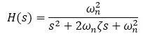
The continuous-time transfer function has two poles and no zeros. The poles can either be real (and may or may not have the same location) or complex conjugate, where the real parts of the poles are identical and imaginary parts are negative to each other.

The poles of the continuous transfer function can be easily determined:

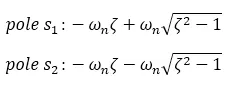
The discrete counterpart of the transfer function is obtained using the zero-order hold technique:

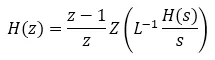
Using a Laplace to Z transform look-up table:

The following is a generic version:

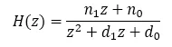
Where:

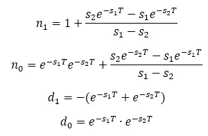
The poles of the discrete transfer function correspond to the poles of the continuous time transfer functions such as:

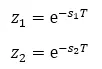
When the zero-order hold technique is used, the natural frequency and damping factor properties of each pole are preserved in the resulting discrete transfer function. This does not hold true for other approximations, such as the Tustin (bilinear) transformation.

The natural frequency and damping ratio of the system poles are defined in the following table (from MATLAB documentation), consistent with the simulation.

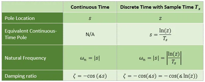
Note: There are many values of "s" for each "z", e.g.

Thus:

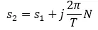
Mapping of continuous-time poles to z-plane

The following table captures the essence of mapping s-plane poles to the z domain.

From Digital Control of Dynamic Systems by Franklin, Powell, and Workman:

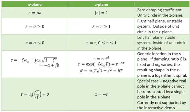
Z-plane overview

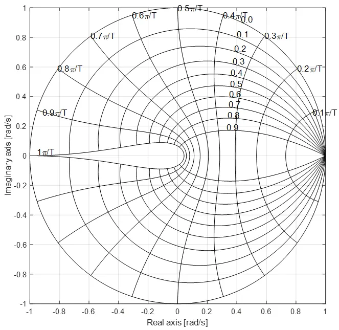
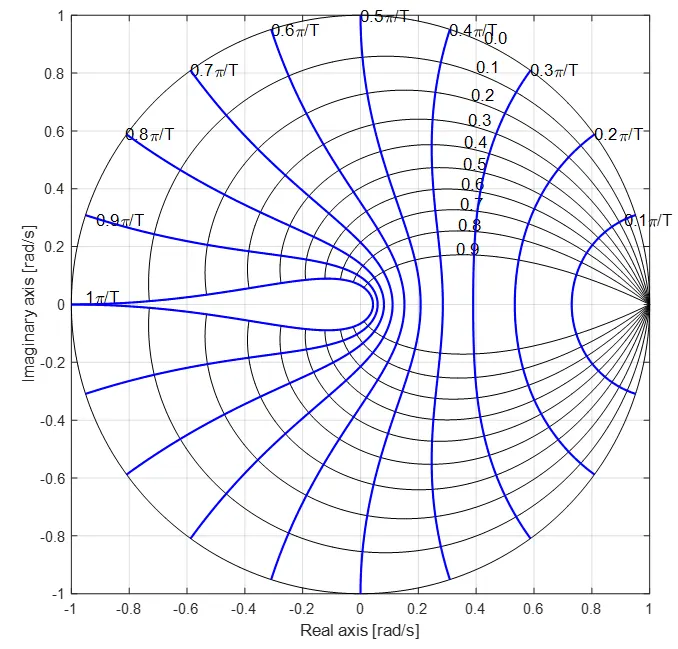
The z-plane below is comprised of a unit circle and a number of lines within. There are two line types? Constant frequency and constant damping ratio.

The dominant feature of the plane is the unit circle- the unit circle is the zero-damping coefficient contour. Systems with any pole outside the unit circle are inherently unstable and of a little use to us. Location outside the unit circle corresponds to negative damping coefficient. However, unlike poles, transfer function zeroes outside the unit circle do not cause system instability.

The plane is symmetrical around the real axis.

Constant Frequency Contours

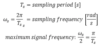
The highlighted lines in the figure below are the constant frequency lines. Frequency is expressed as the distance from the origin in the s-plane. The Z-plane is different, however, since the maximum frequency is limited and defined as two signal samples per sampling period (as per Nyquist sampling theorem).

Hence, the maximum signal frequency is defined as one half of the sampling frequency:

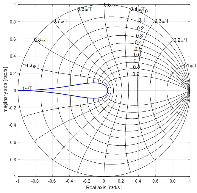
E.g., the sampling period Ts = 0.1 s and the natural frequency is 31.4 rad/s. The poles would therefore be located on the PI/T constraint frequency line, such as shown below. The actual location also depends on the damping factor.

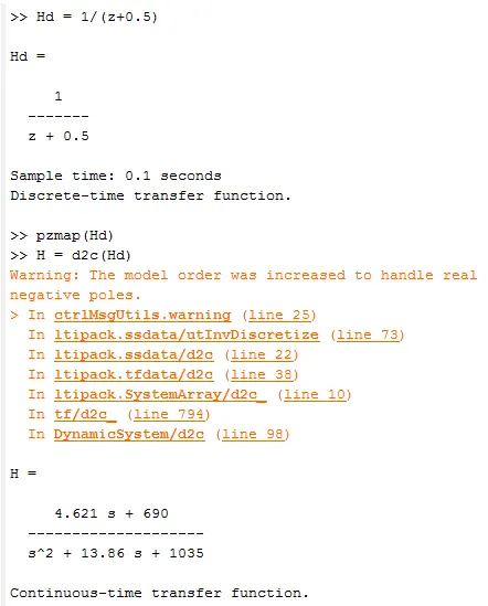
Such poles cannot be represented by a single pole in the z-domain.

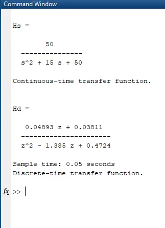
clc;

 clear all;

 format compact;

 close all

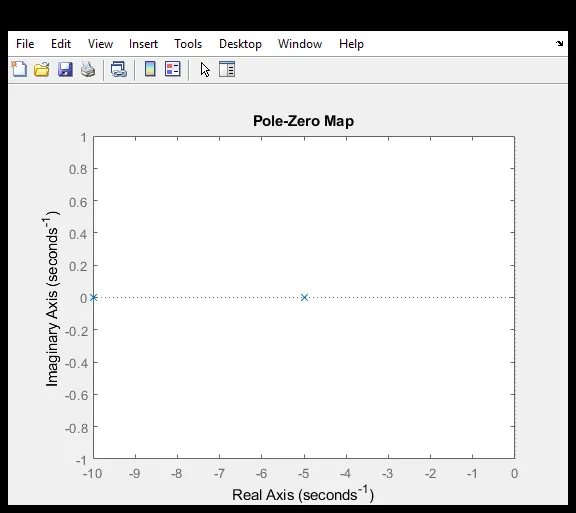
poles = [-10 + 0j, -5 + 0j];

 

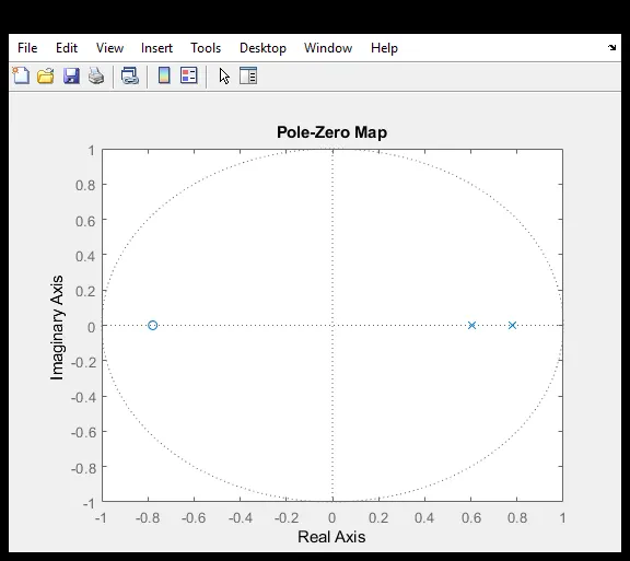
T = 0.05;

 

 

r = poly(poles);

 

Hs = tf(r(end),r)

Hd = c2d(Hs, T, 'zoh')

 

figure(1)

pzmap(Hs)

figure(2)

pzmap(Hd)

figure(3)

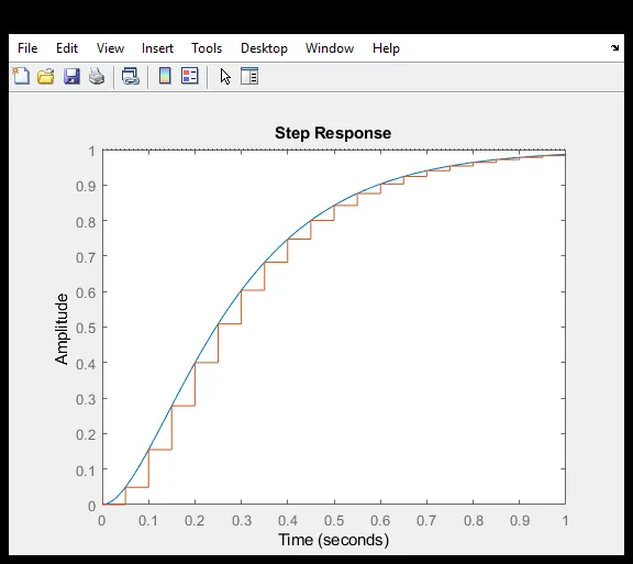
step(Hs, 1)

hold on

step(Hd, 1)

 

Constant Damping Factor Contours -

Constant damping factor contours are shown below. The unit circle in the Z-plane corresponds to the imaginary axis in the Laplace domain. Therefore, the damping coefficient is zero for poles located on the unit circle.

Locations closer to the inner contours in the Z-plane or farther in the left-side in the Laplace-plane correspond to a higher damping factor.

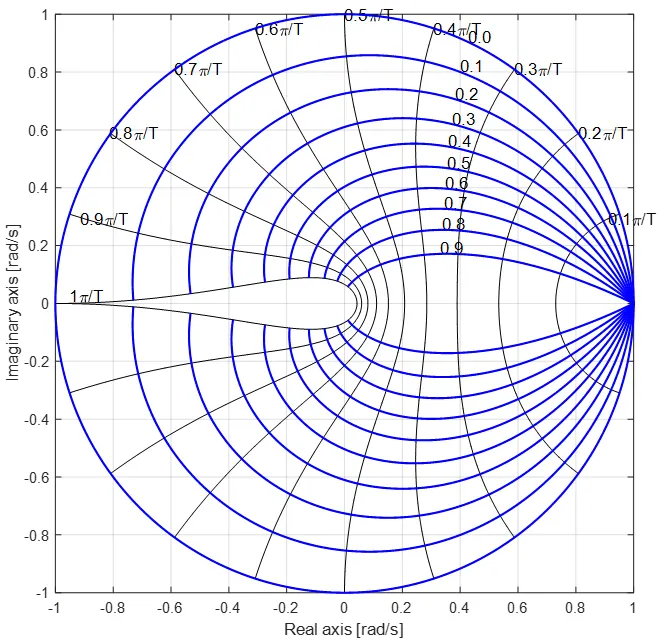
E.g., a version of the transfer function with natural frequency of 12.7 rad/s and damping factor of 0.1 would be:

Or:

The natural frequency of 12.7 rad/s corresponds to the 0.4 PI/T contour line as shown below. The two poles are located at the intersections of the two contours.

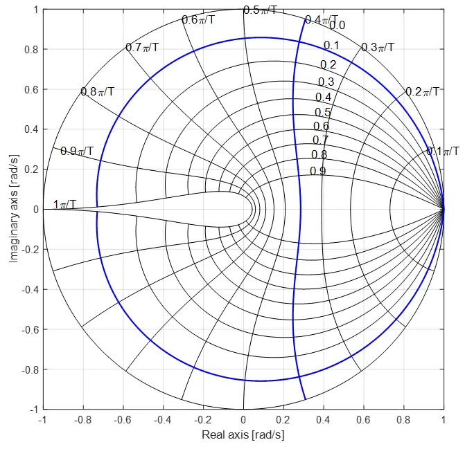
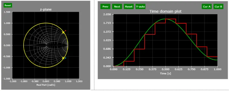
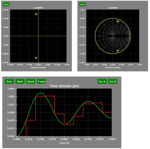
A snapshot of the interactive demo verifies the results: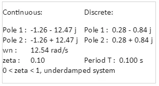

Number of samples per period

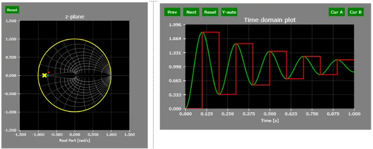
When displayed in the time domain (the interactive example easily allows that by dragging both poles to the -1 location in the z-plane, which coincides with the PI/T contour line), it is shown that the continuous time signal is sampled just twice per period.

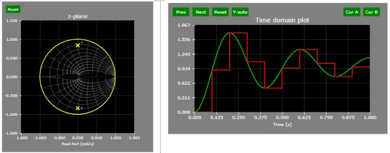
At the 0.5 PI/T contour line, there are four samples per signal period (lower damping coefficient shows the count with more clarity).

At the 0.2 PI/T contour line, there are ten samples per signal period (lower damping coefficient shows the count with more clarity).

Examples are shown below.

PI/T contour line - 2 samples per period:

0.5 PI/T contour line - 4 samples per period:

0.2 PI/T contour line - 10 samples per period: