Bode Plots and Step Response

Week 2 Challenge: Bode Plots and Step Response

Aim –

1. Which are the MATLAB commands related to transfer function, pole-zero-gain and step response? Take an example transfer function and apply all commands.
2. For the unity feedback system shown in figure below

Determine closed loop step response using MATLAB commands. Comment on the result.

3.Explain the MATLAB model ‘scdspeedctrl’. Comment on results for non-tuned PID gain values.

click here scdspeedctrl

4.What is the importance of bode plot for control system design? Using MATLAB make a bode plot of transfer function

1. Which are the MATLAB commands related to transfer function, pole-zero-gain and step response? Take an example transfer function and apply all commands.

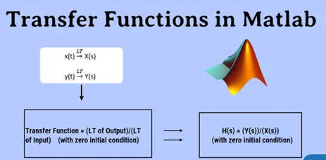
A transfer function is represented by ‘H(s)’. H(s) is a complex function and ‘s’ is a complex variable. It is obtained by taking the Laplace transform of impulse response h(t). transfer function and impulse response are only used in LTI systems. LTI system means Linear and Time invariant system, according to the linear property as the input is zero then output also becomes zero. Therefore, if we do not consider initial conditions are zero then linear property will fail and if the property fails then the system will become non-linear. Because of non-linearity system will become Non-LTI system. And for non-LTI system we cannot define transfer function, therefore, it is mandatory to assume initial conditions are zero.

Definition of Transfer Functions in Matlab

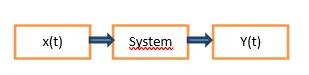
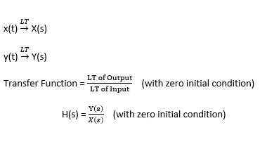
The transfer function of the LTI system is the ratio of Laplace transform of output to the Laplace transform of input of the system by assuming all the initial conditions are zero.

In the above system, the input is x (t) and output is y(t). After taking Laplace Transform of the whole system, x(t) becomes X(s), y(t) becomes Y(s). we consider all the initial conditions are 0 because –

Commands in Transfer function -

Commands	Description
tf	Create tf objects representing continuous time or discrete time transfer functions in polynomial form.
zpk	Create zpk objects representing continuous time or discrete time transfer functions in zero pole gain (factorized) form.
filt	Create tf objects representing discrete time transfer functions using Digital Signal Processing (DSP) convention.

Pole-Zero Gain –

Use zpk to create zero-pole-gain models, or to convert dynamic system models to zero-pole-gain form.

Zero-pole-gain models are a representation of transfer functions in factorized form. For example, consider the following continuous-time SISO transfer function:

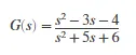
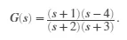
G(s) can be factorized into the zero-pole-gain form as:

A more general representation of the SISO zero-pole-gain model is as follows:

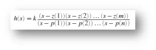
Here, z and p are the vectors of real-valued or complex-valued zeros and poles, and K is the real-valued or complex-valued scalar gain

You can create a zero-pole-gain model object either by specifying the poles, zeros and gains directly, or by converting a model of another type (such as a state-space model ss) to zero-pole-gain form.

You can also use zpk to create generalized state-space models or uncertain state-space ((Robust Control Toolbox)) models.

Step-Response –

The step function is one of most useful functions in MATLAB for control design. Given a system representation, the response to a step input can immediately be plotted. A step input can be described as a change in the input from zero to a finite value at time t = 0. By default, the step command performs a unit step (i.e. the input goes from zero to one at time t = 0). The basic command to use the step function is the following:

step(sys)

This command will produce a series of step response plots, all on the same figure. A plot will be made for each input and output combination. Most problems you will come across in the beginning will be SISO or Single-Input, Single-Output. In this case there will only be one plot made, but the step command handles these problems in the same manner as a SIMO or Single-Input, Multiple-Output.

For example, suppose you want to model a mechanical system consisting of a mass, spring, and damper, with an applied force. You have come up with the transfer function shown below. You wish to see what the system response to unit step input is (an applied force of 1N). To model this, enter the following into MATLAB:

M = 1;

K = 10;

B = 2;

num = 1;

den = [M B K];

sys = tf(num,den);

step(sys)

You should see the following figure:

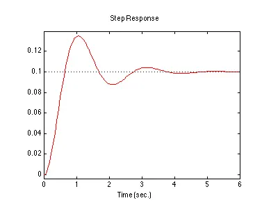
This figure shows the output response, which is the position of the mass. You can see that in steady-state, the mass has moved 0.1m (the spring force balances the applied force). The system is underdamped and has an overshoot.

That's about it for the basic use of the step command. If you are interested, or if you need to use a step command in a more complex format, continue reading.

Changing the magnitude of the step

So far, we have only dealt with unit step inputs. Suppose the input to our system was not 1 Newton but fact 100N. The step command can accommodate this by multiplying the system by 100. For the example above, you should get the following plot

step(100*sys);

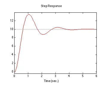
The plot looks similar to the one above it except that the scale on the y-axis is different.

Saving the response

The final note about the step command is that all of the above variations can be used with a left hand arguments. There are two ways to invoke the left hand arguments, depending on whether or not the time vector was used in the step command. If the time vector is used, the command is:

[y,t] = step(sys);

or

[y,t] = step(sys,t);

If the system is in state-space form, all of the states can be returned:

[y,t,x] = step(sys);

The y vector contains the output response. It has as many columns as outputs and as many rows as elements in the time vector, t. The x vector contains the state response. It has as many columns as states and as many rows as elements in the time vector, t. When used with left hand arguments, no plot is drawn for the step command. You will usually want to put a semicolon after the step command when you invoke it with left-hand arguments; otherwise, MATLAB will print out the entire output, state, and time vectors to the command window. You can plot the output response using plot(t,y) or the state response using plot(t,x).

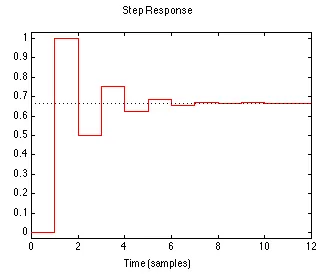
If the system "sys" is a discrete-time system, step will plot the output as piecewise constant. If the sampling time is unspecified, the output time scale will be in samples.

num = 1;

den = [1 0.5];

sys = tf(num,den,-1)

step(sys)

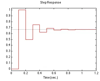
If the sampling time is specified, the time scale will be in seconds.

num = 1;

den = [1 0.5];

Ts = 0.1;

sys = tf(num,den,Ts)

step(sys)

Take an example transfer function and apply all commands.

We will derive transfer function from aa series connected RLC circuit

Consider the RLC circuit –

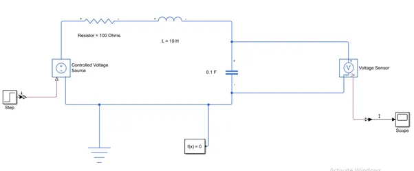
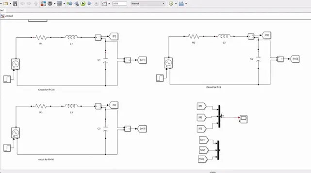
Now using the circuit, we will make Simulation in MATLAB/Simulink.

Now start MATLAB & go to Simulink window.

Now always connect the voltage sensor across the output terminals and as seen above the circuit is ready and we can plot Step response, Impulse response, Nyquist response etc.

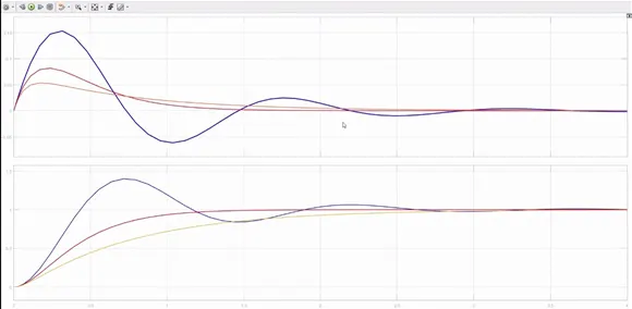
& the response in the scope is –

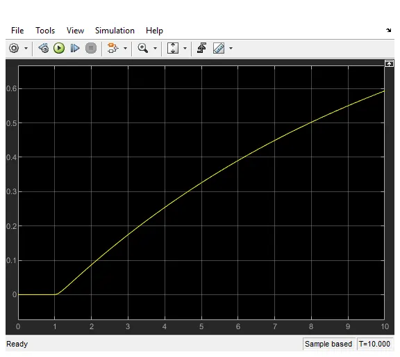
For Transfer function go to command window after performing linear analysis of the RLC we will get the required values for the transfer function & the graphs are shown below –

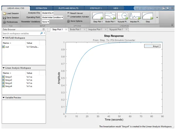
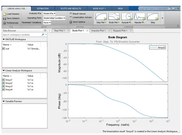
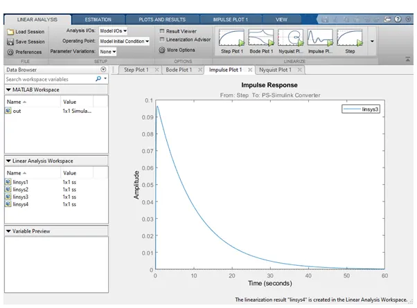
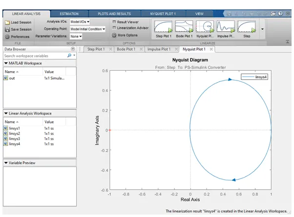
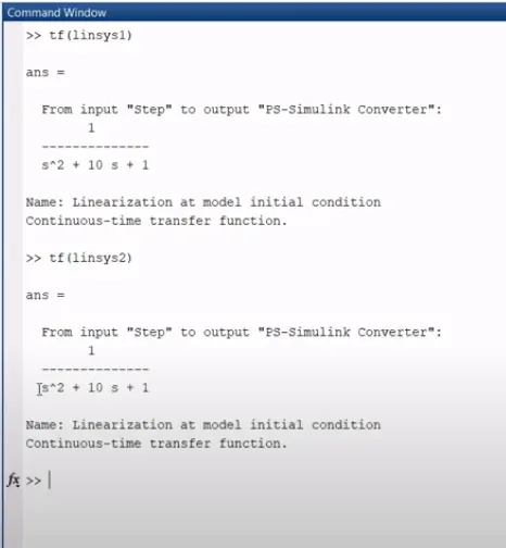
Unit Step Response of RLC circuit –

Plot –

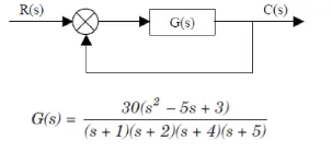
2. For the unity feedback system shown in figure below

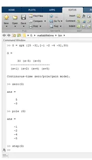
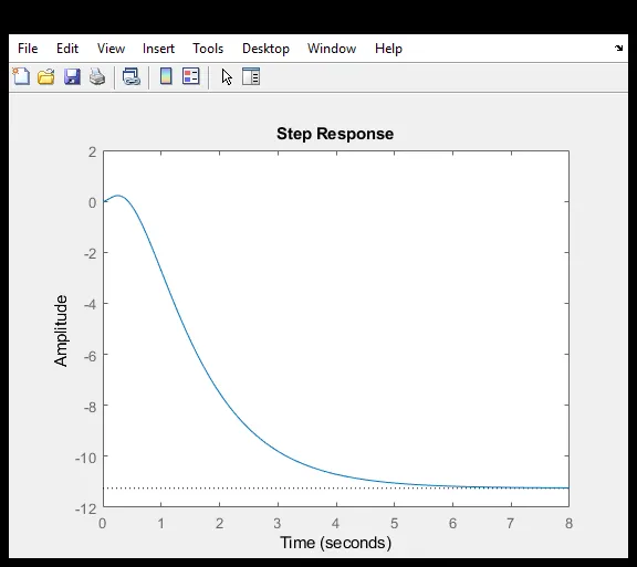
Determine closed loop step response using MATLAB commands. Comment on the result.

Unit Step Response –

The response of a system (with all initial conditions equal to zero at t=0^-, i.e., a zero state response) to the unit step input is called the unit step response. If the problem you are trying to solve also has initial conditions you need to include a zero input response in order to obtain the complete response.

Closed Loop step response -

Owing to the well-recognized fact that model-based control strategies have demonstrated apparently improved system performance of set-point tracking and load disturbance rejection for integrating and unstable processes, e.g., polymerization reactors, heavy bar distillation columns, and steam boilers, control oriented model identification methods have been increasingly explored in the process control community. For safety and economic reasons, integrating and unstable processes are usually not allowed to be operated in an open-loop manner, closed-loop identification methods have therefore been developed in the literature. Step response test has been most widely used for identification in practical applications, owing to its implemental simplicity. Based on closed-loop step test in terms of the internal model control (IMC) structure, Haggblom (1996) ¨ demonstrated that closed-loop identification facilitates better representation of the process dynamic response characteristics for closed-loop operation. Since the pioneering work of using a simple proportional (P) type or proportional-integral-derivative (PID) type controller to stabilize an unstable process for closed loop step test (Deshpande, 1980), closed-loop identification in terms of a low-order controller for stabilization has been preferred for the convenience of implementation. Following the early idea of considering the process time delay as the closed-loop system delay, Ananth and Chidambaram (1999) proposed a first-order-plus-dead-time (FOPDT) model identification method for unstable processes by assigning the dominant closed-loop system pole for fitting. This work has been further extended in the recent papers by using peak values of the closed-loop step response. Using the so-called pseudo-derivative feedback (PDF) for closed-loop stabilization, Paraskevopoulos et al. (2004) developed another FOPDT identification algorithm by constructing amplitude fitting conditions of the closed-loop step response. Based on using the concept of Markov parameters to determine a step response model, Saffer and Doyle (2002) proposed a closed loop identification method for application of model predictive control (MPC).

Plot –

Comment –

This experiment adds feedback to the Open Loop Step Response experiment. The objective is to investigate how feedback changes the system poles and how changes in the pole locations affect the time response of the system. You will estimate such characteristics as settling time, percent overshoot and steady state error. You will verify your calculations through simulations and experiments. Using the MATLAB, you will implement a proportional and derivative controller and will find the system response to a step change in the reference motor position. By comparing the theoretical, simulated and experimental responses you will discover the strengths and limitations of linear modelling.

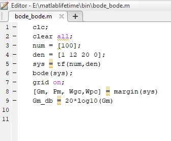
3. What is the importance of bode plot for control system design? Using MATLAB make a bode plot of transfer function

A Bode plot usually consists of magnitude and phase response of a transfer function.

Transfer functions in s-domain quickly become cumbersome to analyse as the control system gets complicated. It’s easy to understand the critical properties of the system by looking at the Bode plot.

1. Bode plot shows the magnitude of gain vs frequency
2. It shows the frequency point at which the gain starts to roll off (called cut off frequency). It gives you the information of the steady state frequency region in which you can operate your control system with good gain.
3. The phase and magnitude response of the loop gain of the control system shows if the system can remain stable at all frequencies of operation. If it is stable, it shows how much margin we have before the system gets unstable. (Phase margin/Gain margin).

Bode Plots are generally used with the Fourier Transform of a given system. An example of a Bode magnitude and phase plot set. The Magnitude plot is typically on the top, and the Phase plot is typically on the bottom of the set. The frequency of the bode plots are plotted against a logarithmic frequency axis. Let’s start from beginning of the subject to understand little deeply…

Control system is a subject where we study the controlling and stabilization of a system in desired manner for any specific purpose. example: Air conditioner is a unit step response first order system with no oscillations, shock absorbers in bike is an example of second order damping system, Traffic light is an open loop system, automatic washing machine is close loop first order undamped system etc.

Now they all are not 100% stable and perfect, there is always a limit and some restrictions to them. when you will go through the subject from beginning to the end you will have to go through 2 things…

1) Response analysis 2) Stability analysis.

Response analysis is the study of transient and steady state characteristics of system which tells how system will perform. like what is peak, delay and rise time, max overshoot, SSR (steady state error), damping, settling time etc. After that we study the stability pact which tells how stable our system is, with the desired characteristics of response requirements. To check stability, Stability methods we use are Routh Hurwitz, polar plot, nyquist plot and Bode Plot and the stability parameters are gain margin, phase margin, roots of TF (transfer function), Location of roots etc. Now, Routh Hurwitz is very limited as it only tells the no. of roots lying at various positions on s-plane only. whereas Polar and nyquist plots can provide us plenty of information regarding GM, PM, Roots etc. regarding stability by which we can analyse relative and absolute both kind of stability and same can be done by BODE PLOT also and in relatively simple manner.

By looking at the Bode plot, we can very get Phase margin, gain margin, TF, Crossover frequencies, system gain, DC gain, Roots and their location by TF, Filter characteristics of system as low pass, high pass or band pass etc., Dominancy like. pole or zero dominant system and many other insights of the system very quickly. With the help of this plot only we can directly comment on the stability of the system without doing any calculations. Bode plots provides relative stability in terms of gain margin and phase margin. It also covers from low frequency to high frequency range. stability in a system can be decreased or increased by feedback circuit. delay circuit, controllers (in time domain), compensators (in frequency domain) etc., so using bode plot only a lot of information regarding stability of system can be drawn out quickly and needed actions can be performed immediately.

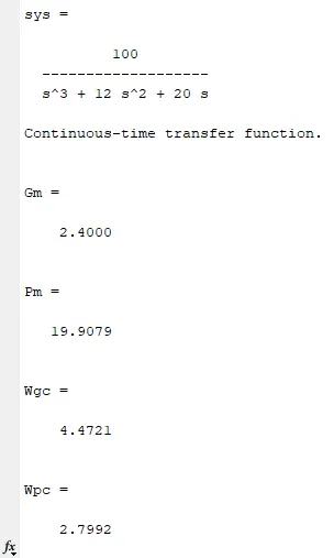
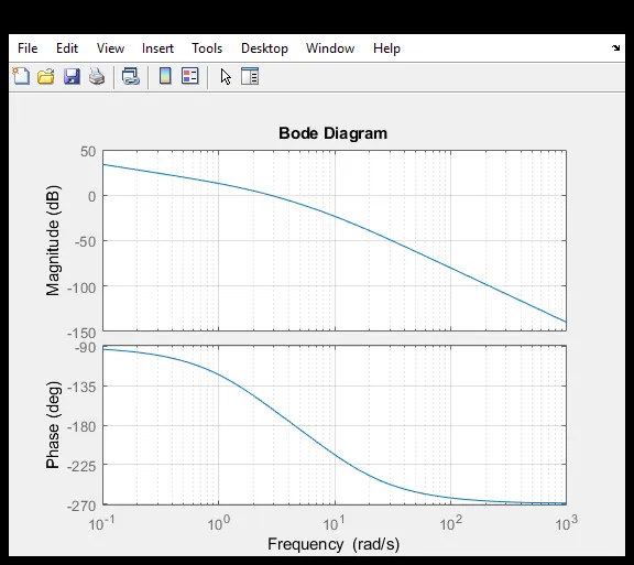
4. Explain the MATLAB model ‘scdspeedctrl’. Comment on results for non-tuned PID gain values.

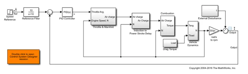
The above model shows the process of designing the single loop control system with both feedback and prefilter compensators & the main aim of this model is to –

1. Track the reference signal from the Simulink step block (Speed Reference) The design requirement is to have a settling time of under 5 seconds and zero steady-state error to the step reference input.
2. Reject an unmeasured output disturbance specified in the subsystem scdspeedctrl/External Disturbance. The design requirement is to reduce the peak deviation to 190 RPM and to have zero steady-state error for a step disturbance input.

Let’s understand the speed control model with the help of simple example –

To start a new design lets first understand the PID controller –

The PID controller is by far the most common control algorithm. Most feedback loops are controlled by this algorithm or minor variations of it. It is implemented in many different forms, as a stand-alone controller or as a part of a DDC (Direct Digital Control) package or a hierarchical distributed process control system. Many thousands of instrument and control engineers worldwide are using such controllers in their daily work. The PID algorithm can be approached from many different directions. It can be viewed as a device that can be operated with a few rules of thumb, but it can also be approached analytically. This chapter gives an introduction to PID control. The basic algorithm and various representations are presented in detail. A description of the properties of the controller in a closed loop based on intuitive arguments is given. The phenomenon of reset windup, which occurs when a controller with integral action is connected to a process with a saturating actuator, is discussed, including several methods to avoid it. Some important aspects of digital computer implementation of PID controllers are given: issues such as prefiltering, different digital approximations, noise filtering, and computer code for good implementation. Operational aspects, such as bumpless transfer between manual and automatic mode and between different parameter sets, are also presented. The chapter ends with some aspects on the use and misuse of PID control with examples of systems where PID control works well and where it does not.

The Feedback Principle –

The idea of feedback is deceptively simple and, yet, extremely powerful. It has had a profound influence on technology. Application of the feedback principle has resulted in major breakthroughs in control, communication, and instrumentation. Many patents have been granted on the idea. Assume for simplicity that the process is such that the process variable increases when the manipulated variable is increased. The principle of feedback can then be expressed as follows: Increase the manipulated variable when the process variable is smaller than the setpoint and decrease the manipulated variable when the process variable is larger than the setpoint. This type of feedback is called negative feedback because the manipulated variable moves in opposite direction to the process variable. The feedback principle can be illustrated by the block diagram shown in Figure 3.1. In this diagram the process and the controller are represented as boxes with arrows denoting inputs and outputs. Notice also that there is a special symbol to denote the summation of signals. The block diagram shows that the process and the controller are connected in a closed feedback loop. The presence of the sign-reversing block indicates that the feedback is negative. The reason why feedback systems are of interest is that feedback makes the process variable close to the setpoint in spite of disturbances and variation of the process characteristics.

When to use PID control?

The requirements on a control system may include many factors, such as response to command signals, insensitivity to measurement noise and process variations, and rejection of load disturbances. The design of a control system also involves aspects of process dynamics, actuator saturation, and disturbance characteristics. It may seem surprising that a controller as simple as the PID controller can work so well. The general empirical observation is that most industrial processes can be controlled reasonably well with PID control provided that the demands on the performance of the control are not too high.

The characteristics of P, I, & D terms –

Increasing the proportional gain has the effect of proportionally increasing the control signal for the same level of error. The fact that the controller will "push" harder for a given level of error tends to cause the closed-loop system to react more quickly, but also to overshoot more. Another effect of increasing is that it tends to reduce, but not eliminate, the steady-state error.

The addition of a derivative term to the controller adds the ability of the controller to "anticipate" error. With simple proportional control, if is fixed, the only way that the control will increase is if the error increases. With derivative control, the control signal can become large if the error begins sloping upward, even while the magnitude of the error is still relatively small. This anticipation tends to add damping to the system, thereby decreasing overshoot. The addition of a derivative term, however, has no effect on the steady-state error.

The addition of an integral term to the controller tends to help reduce steady-state error. If there is a persistent, steady error, the integrator builds and builds, thereby increasing the control signal and driving the error down. A drawback of the integral term, however, is that it can make the system more sluggish (and oscillatory) since when the error signal changes sign, it may take a while for the integrator to "unwind."

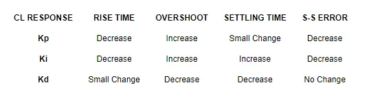
The general effects of each controller parameter on a closed-loop system are summarized in the table below. Note, these guidelines hold in many cases, but not all. If you truly want to know the effect of tuning the individual gains, you will have to do more analysis, or will have to perform testing on the actual system.

Let's first view the open-loop step response. The goal of this problem is to show how each of the above terms contributes to obtaining the common goals of:

1. Fast rise time.
2. Minimal overshoot.
3. Zero steady-state error.

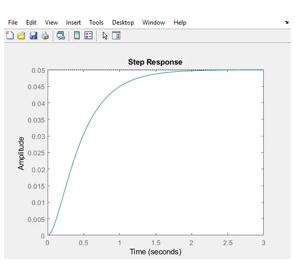
The DC gain of the plant transfer function is 1/20, so 0.05 is the final value of the output to a unit step input. This corresponds to a steady-state error of 0.95, which is quite large. Furthermore, the rise time is about one second, and the settling time is about 1.5 seconds. Let's design a controller that will reduce the rise time, reduce the settling time, and eliminate the steady-state error.

Proportional control –

From the table shown above, we see that the proportional controller (K_p) reduces the rise time, increases the overshoot, and reduces the steady-state error.

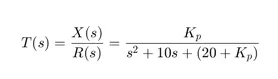
The closed-loop transfer function of our unity-feedback system with a proportional controller is the following, where X(S) is our output (equals Y(s)) and our reference R(S) is the input:

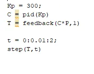
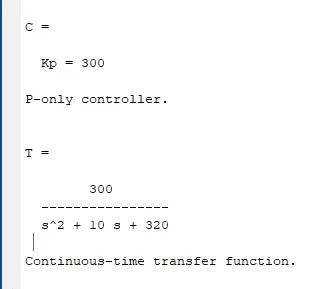
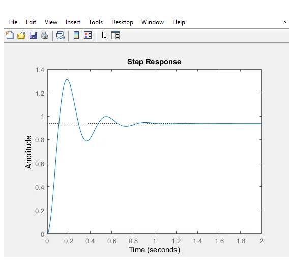
The above plot shows that the proportional controller reduced both the rise time and the steady-state error, increased the overshoot, and decreased the settling time by a small amount.

Proportional Derivative Control –

Now, let's take a look at PD control. Fro

m the table shown above, we see that the addition of derivative control (K_d) tends to reduce both the overshoot and the settling time. The closed-loop transfer function of the given system with a PD controller is:

Let K_p equal 300 as before and let K_d equal 10. Enter the following commands into an m-file and run it in the MATLAB command window.

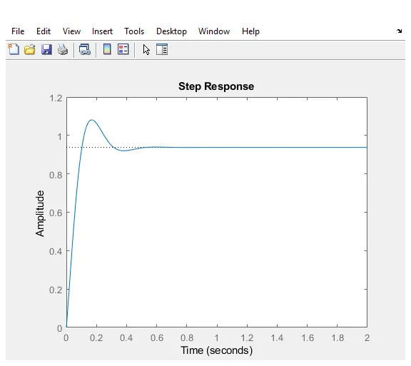
This plot shows that the addition of the derivative term reduced both the overshoot and the settling time, and had a negligible effect on the rise time and the steady-state error.

Proportional – Integral control –

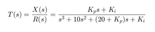
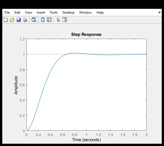
Before proceeding to PID control, let's investigate PI control. From the table, we see that the addition of integral control ( ) tends to decrease the rise time, increase both the overshoot and the settling time, and reduces the steady-state error. For the given system, the closed-loop transfer function with a PI controller is:

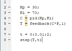
Let's reduce K_p to 30, and let K_i equal 70. Create a new m-file and enter the following commands.

Proportional-Integral Derivative Controller –

Now, let's examine PID control. The closed-loop transfer function of the given system with a PID controller is:

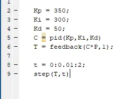
After several iterations of tuning, the gains K_p = 350, K_i = 300, and K_d = 50 provided the desired response. To confirm, enter the following commands to an m-file and run it in the command window. You should obtain the following step response.

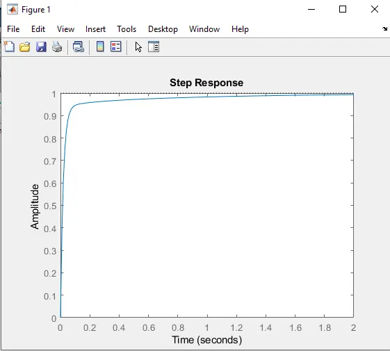
Now, we have designed a closed-loop system with no overshoot, fast rise time, and no steady-state error.

Now we will tune the PID controller –

General Steps to be followed for PID Tuning –

When you are designing a PID controller for a given system, follow the steps shown below to obtain a desired response.

1. Obtain an open-loop response and determine what needs to be improved
2. Add a proportional control to improve the rise time
3. Add a derivative control to reduce the overshoot
4. Add an integral control to reduce the steady-state error
5. Adjust each of the gains K_p, K_i, and K_duntil you obtain a desired overall response. You can always refer to the table shown in this "PID Tutorial" page to find out which controller controls which characteristics.

Lastly, please keep in mind that you do not need to implement all three controllers (proportional, derivative, and integral) into a single system, if not necessary. For example, if a PI controller meets the given requirements (like the above example), then you don't need to implement a derivative controller on the system. Keep the controller as simple as possible.

MATLAB provides tools for automatically choosing optimal PID gains which makes the trial and error process described above unnecessary. You can access the tuning algorithm directly using pidtune or through a nice graphical user interface (GUI) using pidTuner.

The MATLAB automated tuning algorithm chooses PID gains to balance performance (response time, bandwidth) and robustness (stability margins). By default, the algorithm designs for a 60-degree phase margin.

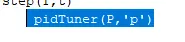
Let's explore these automated tools by first generating a proportional controller for the mass-spring-damper system by entering the command shown below. In the shown syntax, P is the previously generated plant model, and 'p' specifies that the tuner employ a proportional controller.

The pidTuner GUI window, like that shown below, should appear.

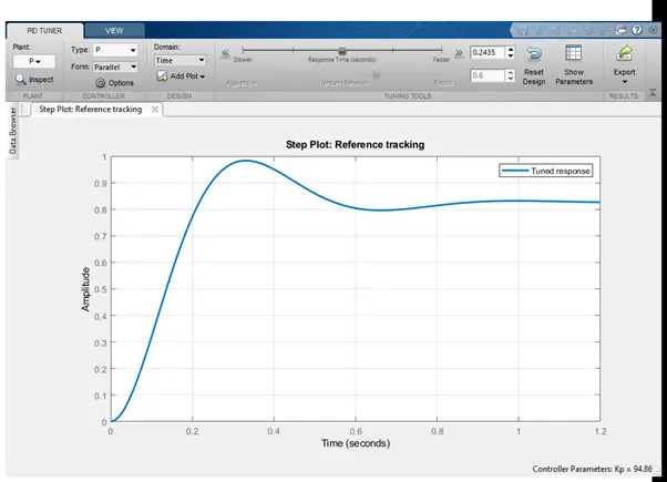
Notice that the step response shown is slower than the proportional controller we designed by hand. Now click on the Show Parameters button on the top right. As expected, the proportional gain, K_p, is smaller than the one we employed, K_p = 94.86 < 300.

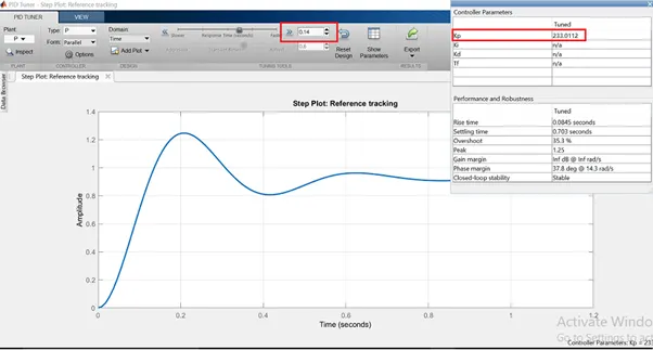
We can now interactively tune the controller parameters and immediately see the resulting response in the GUI window. Try dragging the Response Time slider to the right to 0.14 s, as shown in the figure below. This causes the response to indeed speed up, and we can see K_p is now closer to the manually chosen value. We can also see other performance and robustness parameters for the system. Note that before we adjusted the slider, the target phase margin was 60 degrees. This is the default for the pidTuner and generally provides a good balance between robustness and performance.

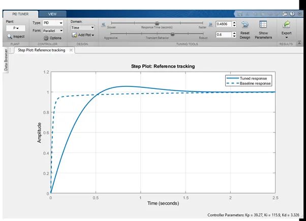
We see in the output window that the automated controller responds slower and exhibits more overshoot than the baseline. Now choose the Domain: Frequency option from the toolstrip, which reveals frequency domain tuning parameters.

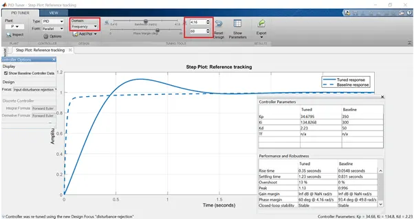
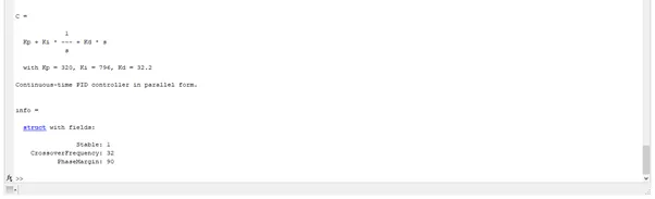
Now type in 32 rad/s for Bandwidth and 90 deg for Phase Margin, to generate a controller similar in performance to the baseline. Keep in mind that a higher closed-loop bandwidth results in a faster rise time, and a larger phase margin reduces the overshoot and improves the system stability.

Finally, we note that we can generate the same controller using the command line tool pidtune instead of the pidTuner GUI employing the following syntax.