Week 4 Challenge: PID Controllers

Week 4 Challenge: PID Controllers

1. In which situations feedforward control of DC motor fails? Prepare a MATLAB script for feedforward control and test it.
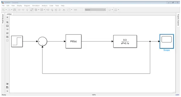
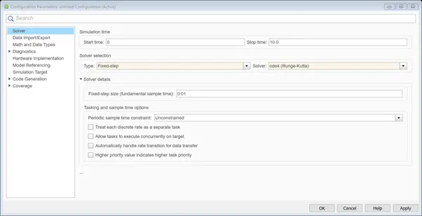
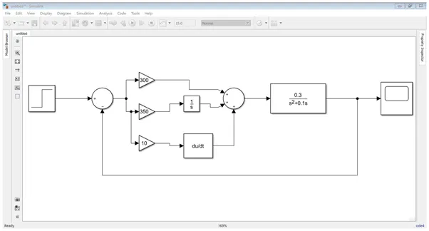
2. Assume a plant and controller. Using MATLAB PID controller block verify system response with General Observation for PID gain. Consider below system

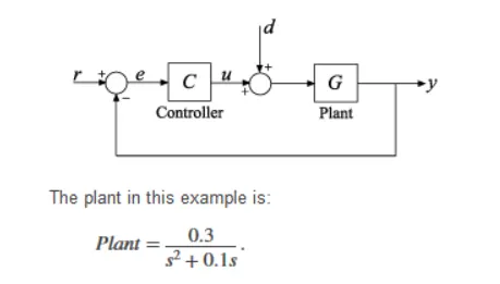
3. Use MATLAB PID tuner and prepare a table showing PID values with response time and transient behaviour coefficient.

1. In which situations feedforward control of DC motor fails? Prepare a MATLAB script for feedforward control and test it.

Situations where Feedforward control of a D.C. Motor fails –

1. Correct mathematical model should be known for exact disturbance rejection.
2. Feedforward controller structure will change with disturbance type & sensor used.
3. Recommended for slow varying process only.
4. Feedforward control alone cannot give desired response hence it always has to be used with feedback controller.
5. The disturbance variables must be measured on-line. In many applications, this is not feasible.
6. To make effective use of feedforward control, at least an approximate process model should be available. In particular, we need to know how the controlled variable responds to changes in both the disturbance and manipulated variables. The quality of feedforward control depends on the accuracy of the process model.
7. Ideal feedforward controllers that are theoretically capable of achieving perfect control may not be physically realizable. Fortunately, practical approximations of these ideal controllers often provide very effective control.

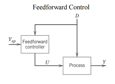
Therefore, it is recommended to use feedforward control system only in following cases –

1. Use cascade first
2. Use feedforward when

– Disturbance can be isolated

– There is no “inner loop” variable that responds to the manipulated variable

– Cannot use the same valve to control the disturbance

In armature controlled D.C. Motor, the applied voltage V_a controls the angular velocity w of the shaft.

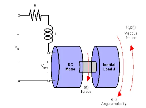
This example shows two DC motor control techniques for reducing the sensitivity of w to load variations (changes in the torque opposed by the motor load).

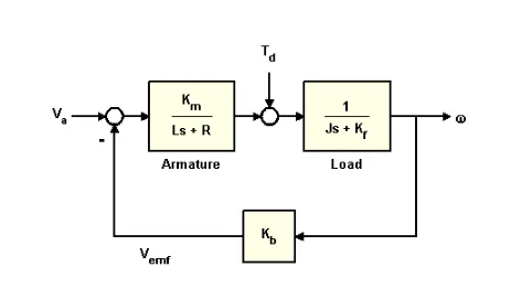
This example shows two DC motor control techniques for reducing the sensitivity of w to load variations (changes in the torque opposed by the motor load).

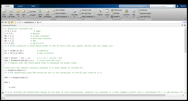
%Physical constants are -

R = 2.0;                % Ohms

L = 0.5;                % Henrys

Km = 0.1;               % torque constant

Kb = 0.1;               % back emf constant

Kf = 0.2;               % Nms

J = 0.02;               % kg.m^2/s^2

% First construct a state-space model of the DC motor with two inputs (Va,Td) and one output (w):

 

h1 = tf(Km,[L R]);            % armature

h2 = tf(1,[J Kf]);            % eqn of motion

 

dcm = ss(h2) * [h1 , 1];      % w = h2 * (h1*Va + Td)

dcm = feedback(dcm,Kb,1,1);   % close back emf loop

 % Compute with the state-space form to minimize the model order.

 

% Now plot the angular velocity response to a step change in voltage Va:

stepplot(dcm(1));

% The feedforward gain Kff should be set to the reciprocal of the DC gain from Va to w.

 

Kff = 1/dcgain(dcm(1))

 

Kff =

 

    4.1000

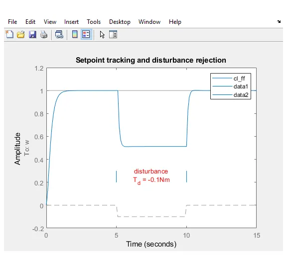
  % To evaluate the feedforward design in the face of load disturbances, simulate the response to a step command w_ref=1 with a disturbance Td = -0.1Nm between t=5 and t=10 seconds:

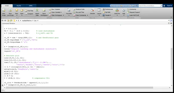
t = 0:0.1:15;

Td = -0.1 * (t>5 & t<10);       % load disturbance

u = [ones(size(t)) ; Td];       % w_ref=1 and Td

 

cl_ff = dcm * diag([Kff,1]);    % add feedforward gain

cl_ff.InputName = {'w_ref','Td'};

cl_ff.OutputName = 'w';

h = lsimplot(cl_ff,u,t);

title('Setpoint tracking and disturbance rejection')

legend('cl\_ff')

 

% Annotate plot

line([5,5],[.2,.3]);

line([10,10],[.2,.3]);

text(7.5,.25,{'disturbance','T_d = -0.1Nm'},...

'vertic','middle','horiz','center','color','r');

h = rlocusplot(tf(1,[1 0]) * dcm(1));

setoptions(h,'FreqUnits','rad/s');

xlim([-15 5]);

ylim([-15 15]);
 K = 5;

C = tf(K,[1 0]);            % compensator K/s

 

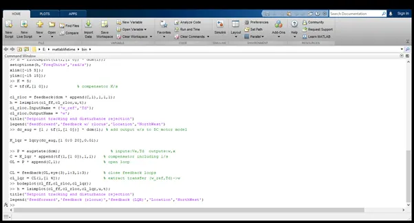
cl_rloc = feedback(dcm * append(C,1),1,1,1);

h = lsimplot(cl_ff,cl_rloc,u,t);

cl_rloc.InputName = {'w_ref','Td'};

cl_rloc.OutputName = 'w';

title('Setpoint tracking and disturbance rejection')

legend('feedforward','feedback w/ rlocus','Location','NorthWest')

dc_aug = [1 ; tf(1,[1 0])] * dcm(1); % add output w/s to DC motor model

 

K_lqr = lqry(dc_aug,[1 0;0 20],0.01);

 

P = augstate(dcm);                     % inputs:Va,Td  outputs:w,x

C = K_lqr * append(tf(1,[1 0]),1,1);   % compensator including 1/s

OL = P * append(C,1);                  % open loop

 

CL = feedback(OL,eye(3),1:3,1:3);      % close feedback loops

cl_lqr = CL(1,[1 4]);                  % extract transfer (w_ref,Td)->w

bodeplot(cl_ff,cl_rloc,cl_lqr);

h = lsimplot(cl_ff,cl_rloc,cl_lqr,u,t);

title('Setpoint tracking and disturbance rejection')

legend('feedforward','feedback (rlocus)','feedback (LQR)','Location','NorthWest')

%Physical constants are -

R = 2.0;                % Ohms

L = 0.5;                % Henrys

Km = 0.1;               % torque constant

Kb = 0.1;               % back emf constant

Kf = 0.2;               % Nms

J = 0.02;               % kg.m^2/s^2

% First construct a state-space model of the DC motor with two inputs (Va,Td) and one output (w):

h1 = tf(Km,[L R]);            % armature

h2 = tf(1,[J Kf]);            % eqn of motion

 

dcm = ss(h2) * [h1 , 1];      % w = h2 * (h1*Va + Td)

dcm = feedback(dcm,Kb,1,1);   % close back emf loop

% Compute with the state-space form to minimize the model order.

 

% Now plot the angular velocity response to a step change in voltage Va:

stepplot(dcm(1));

% The feedforward gain Kff should be set to the reciprocal of the DC gain from Va to w.

Kff = 1/dcgain(dcm(1))
Kff =

 

    4.1000

 

% To evaluate the feedforward design in the face of load disturbances, simulate the response to a step command w_ref=1 with a disturbance Td = -0.1Nm between t=5 and t=10 seconds:

 

t = 0:0.1:15;

Td = -0.1 * (t>5 & t<10);       % load disturbance

u = [ones(size(t)) ; Td];       % w_ref=1 and Td

 

cl_ff = dcm * diag([Kff,1]);    % add feedforward gain

cl_ff.InputName = {'w_ref','Td'};

cl_ff.OutputName = 'w';

 

h = lsimplot(cl_ff,u,t);

title('Setpoint tracking and disturbance rejection')

legend('cl\_ff')

 

% Annotate plot

line([5,5],[.2,.3]);

line([10,10],[.2,.3]);

text(7.5,.25,{'disturbance','T_d = -0.1Nm'},...

            'vertic','middle','horiz','center','color','r');

h = rlocusplot(tf(1,[1 0]) * dcm(1));

setoptions(h,'FreqUnits','rad/s');

xlim([-15 5]);

ylim([-15 15]);

K = 5;

C = tf(K,[1 0]);            % compensator K/s

 

cl_rloc = feedback(dcm * append(C,1),1,1,1);

h = lsimplot(cl_ff,cl_rloc,u,t);

cl_rloc.InputName = {'w_ref','Td'};

cl_rloc.OutputName = 'w';

title('Setpoint tracking and disturbance rejection')

legend('feedforward','feedback w/ rlocus','Location','NorthWest')

dc_aug = [1 ; tf(1,[1 0])] * dcm(1); % add output w/s to DC motor model

 

K_lqr = lqry(dc_aug,[1 0;0 20],0.01);

 

P = augstate(dcm);                     % inputs:Va,Td  outputs:w,x

C = K_lqr * append(tf(1,[1 0]),1,1);   % compensator including 1/s

OL = P * append(C,1);                  % open loop

 

CL = feedback(OL,eye(3),1:3,1:3);      % close feedback loops

cl_lqr = CL(1,[1 4]);                  % extract transfer (w_ref,Td)->w

bodeplot(cl_ff,cl_rloc,cl_lqr);

h = lsimplot(cl_ff,cl_rloc,cl_lqr,u,t);

title('Setpoint tracking and disturbance rejection')

legend('feedforward','feedback (rlocus)','feedback (LQR)','Location','NorthWest')

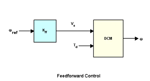
Feedforward Control –

Clearly feedforward control handles load disturbances poorly.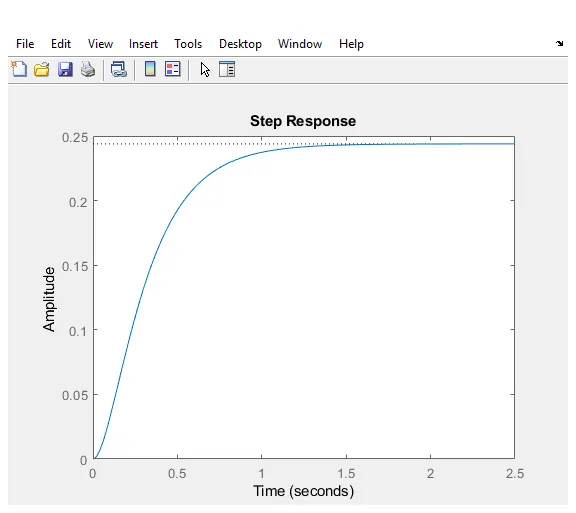

Feedforward Control -

Feedback DC Motor Control Design

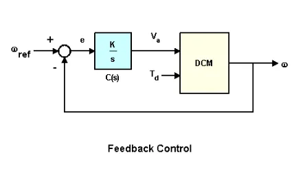
To enforce zero steady-state error, use integral control of the form

C(s) = K/s

where K is to be determined.

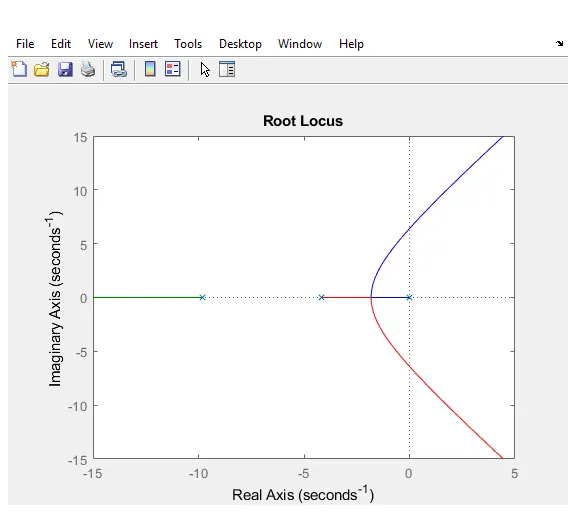
To determine the gain K, you can use the root locus technique applied to the open-loop 1/s * transfer(Va->w):

Click on the curves to read the gain values and related info. A reasonable choice here is K = 5. Note that the SISO Design Tool offers an integrated GUI to perform such designs (help sisotool for details).

Compare this new design with the initial feedforward design on the same test case:

Compare this new design with the initial feedforward design on the same test case:

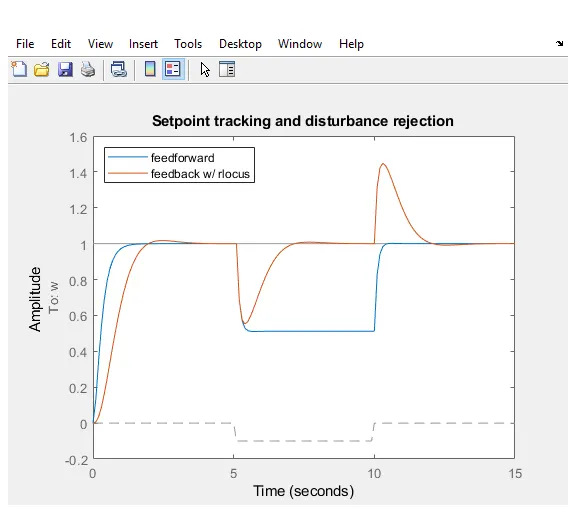
The root locus design is better at rejecting load disturbances.

LQR DC Motor Control Design

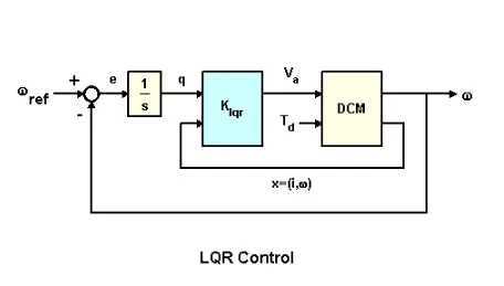
To further improve performance, try designing a linear quadratic regulator (LQR) for the feedback structure shown below.

In addition to the integral of error, the LQR scheme also uses the state vector x=(i,w) to synthesize the driving voltage Va. The resulting voltage is of the form

Va = K1 * w + K2 * w/s + K3 * i

where i is the armature current.

For better disturbance rejection, use a cost function that penalizes large integral error, e.g., the cost function

Where,

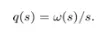
The optimal LQR gain for this cost function is computed as follows:

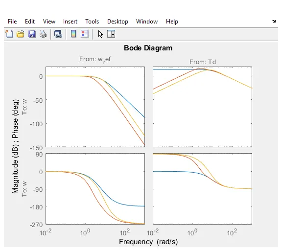
Click on the curves to identify the systems or inspect the data.

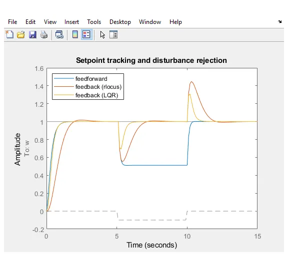
Because of additional degrees of freedom, the LQR compensator performs best at rejecting load disturbances (among the three DC motor control designs discussed here).

Now Lets take a Heat Exchanger Model in MATLAB -

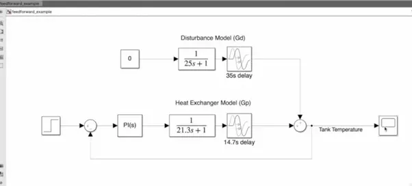
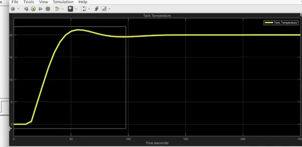
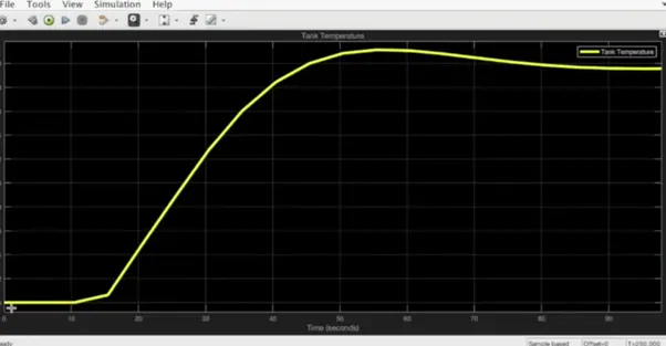
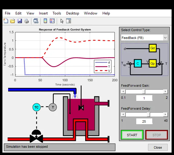
for a fixed inlet temperature if we want to raise the tank temperature by 20 degrees it would take about 15 secs. to start warming up & then about another 25 to 40 seconds or so to reach the commanded temperature so our feedback controller does a pretty good job. But once we are at steady state, Let’s say the inlet temperature drops suddenly by 10 degrees, this disturbance would ripple through & cause a tank temperature variation that the feedback controller would remove slowly but not before there was a large temperature drop in the tank.

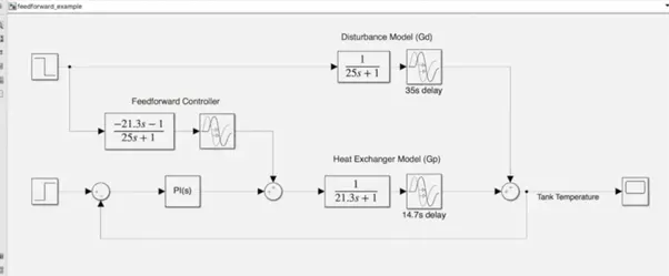
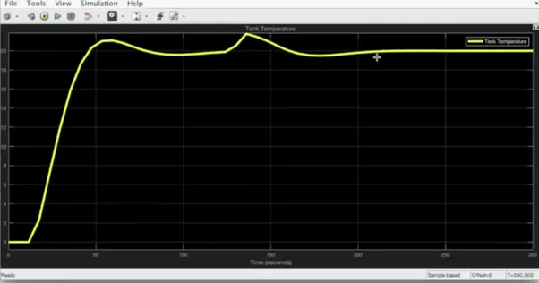
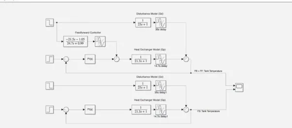
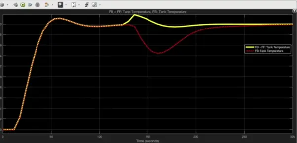
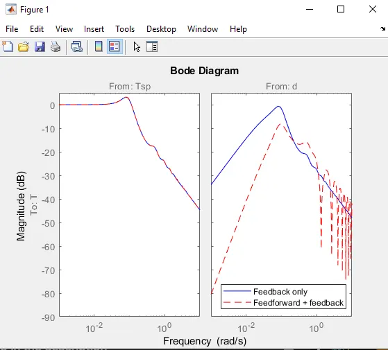
So now lets see how adding feebforward control on the disturbance path can help this so we can measure the inlet fluid temperature and adjust our controller output to start adding heat to the tank before the tank temperature gets affected. Remember our feedforward controller can be calculated as the negative ratio of GD over GP in our case this is saying that about 20 seconds after we measure the disturbance then we want to start adjusting the steam valve per this transfer function. Then we will add heat into the system that will cancel the heat removed by the cold fluid & now if we run this simulation you will see that there is indeed the case very little devaiation from steady state however, since we are working with models we know them perfectly then we are able to cancel out the disturbance really well with real hardware so feedforward can only reduce this impact & not move it completely & we can demonstrate this by changinf the feedforward controller parameters slightly, now when we run this disturbance, we will have a larger effect on the tank temperature but still not as much as the feedback control loop system. so we will duplicate the syatem & remove feedforward controller in one of them so that we can compare before and after. Notice that feeding forward the disturbance didn’t change the way the system reacts to set point changes, we haven’t changed the way system will respond to commands only to disturbances & that’s pretty cool. In heat exchanger model, it will bring up an interactive GUI that will let you switch controllers between feedback only and feedback + feedforward so you can get more intuitive feel for how all of this is working.

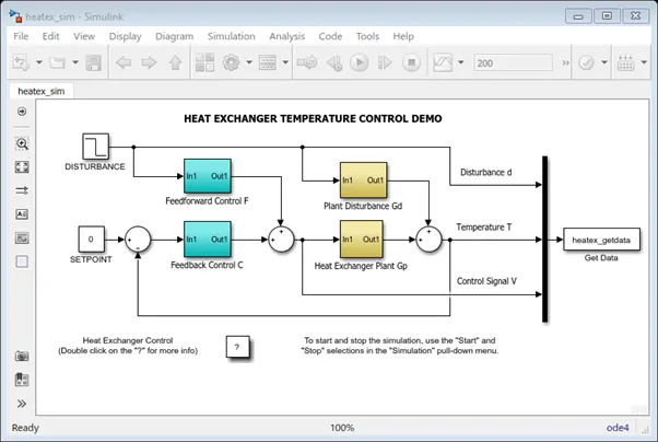
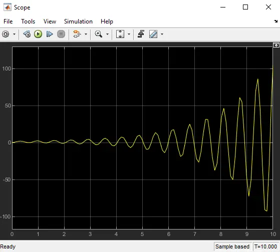
2. Assume a plant and controller. Using MATLAB PID controller block verify system response withGeneral Observation for PID gain. Consider below system.

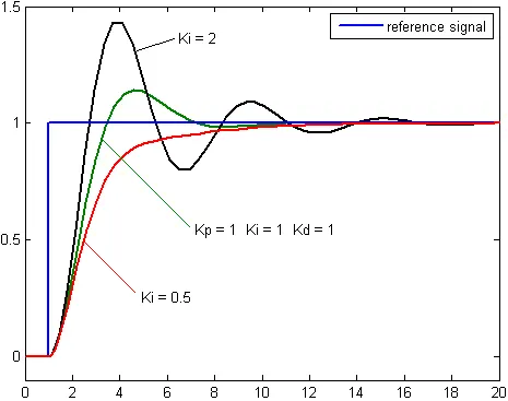
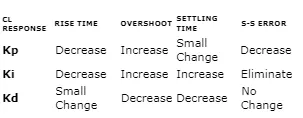
The proportional term, K_p, is entirely based on the error and that, let's say, double the error would mean doubling K_p (applying proportional force). This therefore implies that increasing K_p is a result of the system heading in the wrong direction so K_p is increased to ensure the system goes on the right direction or at least tries to reduce the error as time passes so an increase in K_p would affect the system in such a way to adjust the heading of the system so it stays on the right path.

The derivative term, K_d, is based on the rate of change of the error so an increase in K_d implies that the rate of change of error has increased over time so double the error would result in double the force. An increase by double the change in the system's heading would take place if the system's heading is doubled in error from the previous feedback result. K_d causes the system to react faster as the error increases.

An increase in the integral term, K_i, means that the error is increased over time. The integral accounts for the sum of error over time. Even a small increase in the error would increase the integral so the system would have to head in the right direction for an equal amount of time for the integral to balance to zero.

3. Use MATLAB PID tuner and prepare a table showing PID values with response time and transient behaviour coefficient.

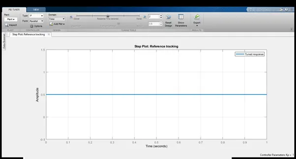
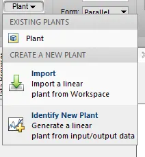
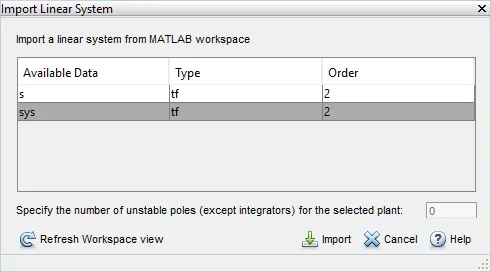
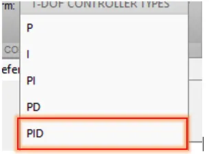
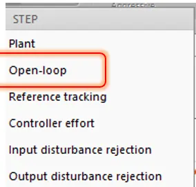
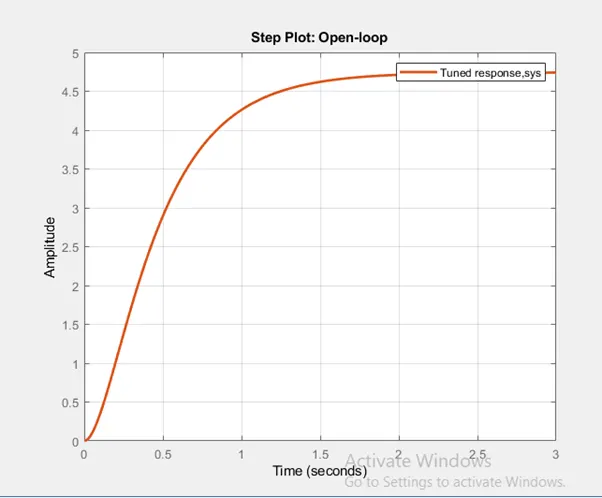
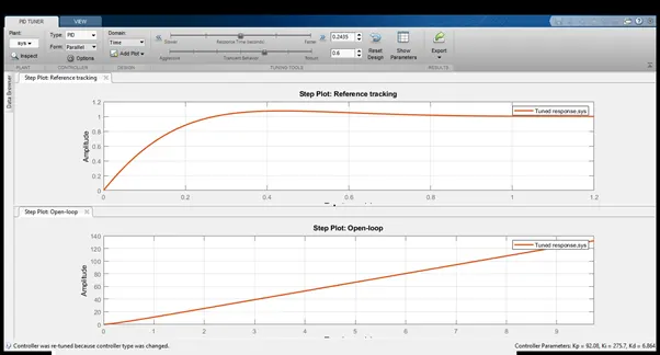
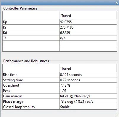
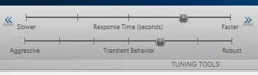
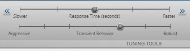
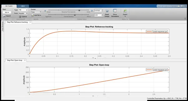
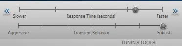
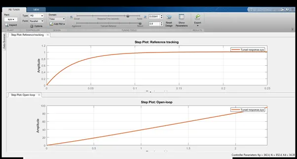
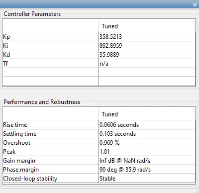
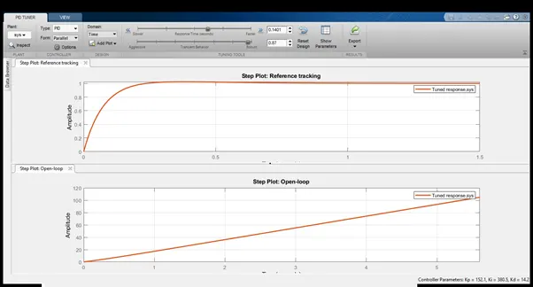
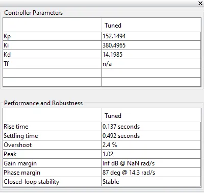
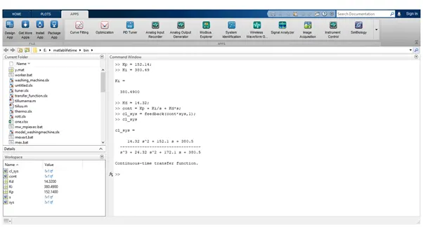
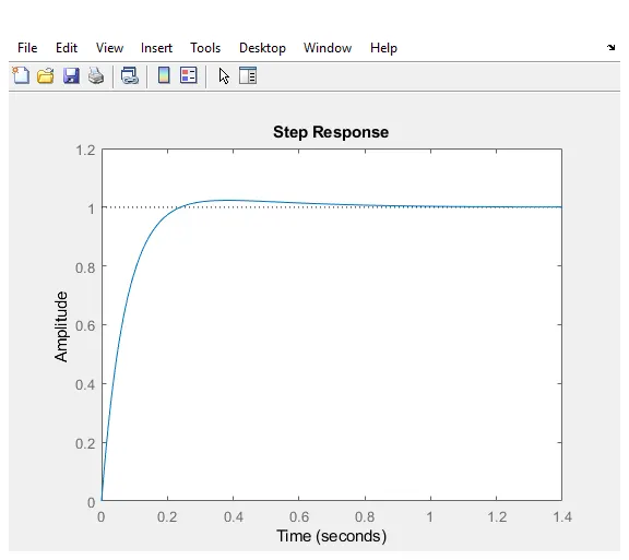
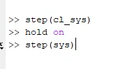
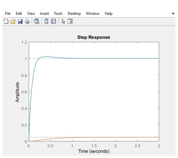
You can use PID Tuner to interactively tune PID gains in a Simulink^® model containing a PID Controller, Discrete PID Controller, PID Controller (2DOF), or Discrete PID Controller (2DOF) block.

Prerequisites for PID Tuning

Before you can use PID Tuner, you must:

• Create a Simulink model containing a PID Controller, Discrete PID Controller, PID Controller (2DOF), or Discrete PID Controller (2DOF) block. Your model can have one or more PID blocks, but you can only tune one PID block at a time.
  • If you are tuning a multi-loop control system with coupling between the loops, consider using other Simulink Control Design™ tools instead of PID Tuner. For more information, see choose a control design approach.
  • The PID Controller blocks support vector signals. However, using PID Tunerrequires scalar signals at the block inputs. That is, the PID block must represent a single PID controller.

Your plant (all blocks in the control loop other than the controller) can be linear or nonlinear. The plant can also be of any order, and have any time delays.

1. Configure the PID block settings, such as controller type, controller form, time domain, sample time. For more information on these block settings, see the individual block reference pages:
2. PID Controller.
3. Discrete PID Controller.
4. PID Controller (2 DOF)
5. Discrete PID Controller (2 DOF)

Opening PID Tuner-

To open PID Tuner and view the initial compensator design:

1. Open the Simulink model by typing the model name at the MATLAB^®command prompt.
2. To open the block dialog box, double-click the PID controller block.
3. In the block dialog box, in the Select Tuning Methoddrop-down list, select Transfer Function Based (PID Tuner App). To open PID Tuner, click Tune.

When you open PID Tuner, the following actions occur:

4. PID Tunerautomatically linearizes the plant at the operating point specified by the model initial conditions, as described in what plant does PID tuner see?. If you want to design a controller for a different operating point, see tune at a different operating pouint.
5. PID Tunercomputes an initial compensator design for the linearized plant model using the algorithm described in PID Tuning Algorithm.
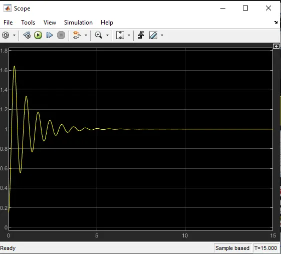
6. PID Tunerdisplays the closed-loop step reference tracking response for the initial compensator design. For comparison, the display also includes the closed-loop response for the gains specified in the PID controller block, if that closed loop is stable, as shown in the following figure.