Week 10: Modeling and Simulation of flow around an Ahmed Body

AIM:

• To simulate the flow over the Ahmed body.
• To understand the domain creation for external aerodynamics simulation.

THEORY:

Ahmed body is an aerodynamic shape invented in 1984 to reduce the drag of automotive vehicles. Later on, Ahmed's body becomes a test case to validate the solver using experimental results(Wind Tunnel results) compared with simulation results. This Ahmed body is one reason to have an aerodynamic shape in automotive vehicles. This shape reduces the large consumption fule and also increases the mileage of vehicles.

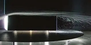
The above image describes the flow over Ahmed's body with smoke visualization in a wind tunnel.

PROCEDURE FOR SETTING UP THE SIMULATION CASE:

CREATING AHMED BODY USING CAD SOFTWARE:

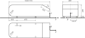
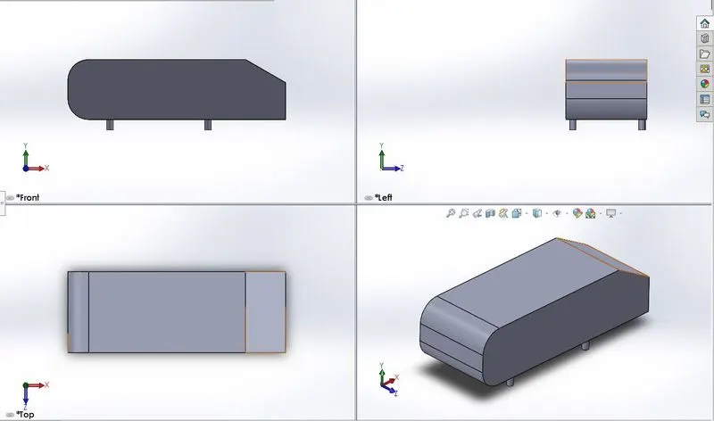
Here I have used Solidworks to design Ahmed body.

Importing Geometry, Creating Virtual Wind Tunnel & Diagnosis:

• I have used Solidworks to design the airfoil and domain and converted it into an STL file.
• Import the geometry in the STL file which is in the form of triangles.
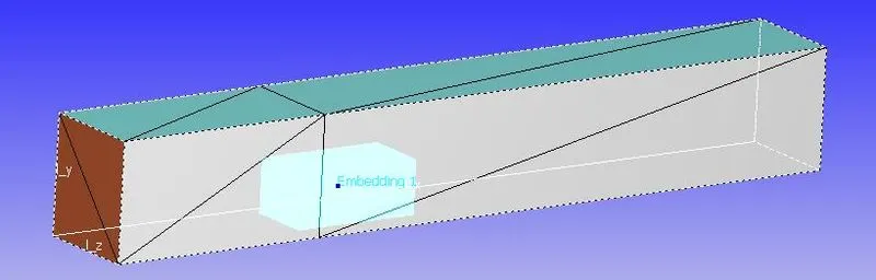
• Here I have calculated the domain size, the front side is 3 times greater than the length of the test object and the backside is 5 times greater than the test object.
• We are having a large length at the backside is due to capture wake produced and to settle down gives accurate results.
• Calculating the distance of boundary layer growth in the given statement boundary layer thickness should be 30mm and 400 mm in front of the body.
• Approximation of boundary layer can be defined by
• `delta approx (0.382*x)/(Rex^0.2)`
• We know that `delta` is 0.003.
• We can also calculate the Reynolds number using`Re=(rho*V*L)/(mu)`.
• Finally, we get the value for `x=1.66m`, this 1.66 + 0.4 = 2.04m is considered as slip region.
• After importing run the diagnosis for checking the geometry for any problem in cad.
• Most important this that we need to check the normal also, the normal should be pointing towards the domain.

Case set-up :

• The application type is Timebase.
• A predefined air mixture is used.
• Using turbulent Prandtl number 0.9.
• Using turbulent Schmidt number 0.78.
• O2 and N2 are species of air.

Simulation Parameters:

• A transient-state solver is used.
• End time can be calculated, End time = length of the domain/velocity.
• We get End time = 0.1827, which is the one cycle.
• We are going to run the simulation 4 cycle then `4*0.1827 approx 0.7s`
• The minimum time step is 1e-9s.
• The maximum time step is 1s.

Boundary Condition and Region Initialization:

• The Inlet, Outlet, Top and sidewall, Slip region, Bottom wall, and Ahmed body total of seven boundaries are used.
• Inlet and velocity inlet and velocity as 40 m/s and species as air.
• Outlet as pressure outlet of 101325 pa and backflow species as air.
• The top and sidewall are considered as Symmetry.
• The Slip region is considered a slip region.
• The bottom wall is considered a wall as the law of wall.
• The Ahmed body is considered a wall and the law of wall condition are provided.
• In Region & Initialization, we are creating a region for fluid flow and setting the velocity as 40m/s.

Physical Model:

• We are using the k−ωSST turbulence model, which has automatic wall treatment.

Grid Control:

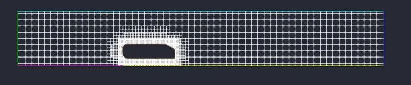
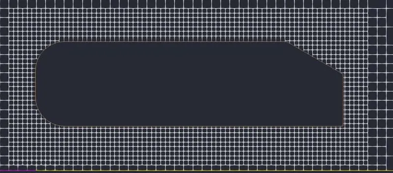
• In grid control, we will be defining the mesh size for the domain (0.002 m is the mesh size).
• Here we are using fixed embedding to refine the mesh to capture the flow physics.
• In fixed embedding, we are using the box method which will create a boundary over the test object.
• If you see that the boundary will have well-refined mesh but outside the mesh well be coarse mesh.

Output and Post-processing:

• In the post-variable selection, we can select the output that we need for post-processing.
• In output files, we can set time intervals for writing the 3D output.
• We can also set time intervals for writing, restarting files.

Running Simulation:

• After finishing setting up the simulation case we need to export the input files in a folder.
• Now open the Cygwin terminal and navigate to the folder where you exported the input files.
• Now run the executable mpiexec.exe -n 2 converge.exe restricted.
• After finishing the simulation we need to convert the output file to paraview format.
• mpiexec.exe -n 2 post_convert_30_msmpi_64.exe command is used to convert the file as ParaView format.

RESULTS:

MESH GENERATION:

VELOCITY CONTOUR:

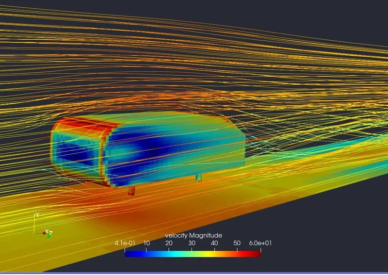
VELOCITY OVER THE AHMED BODY:

VELOCITY STREAMLINES:

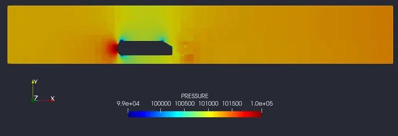
PRESSURE CONTOUR:

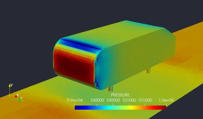
PRESSURE OVER THE BODY:

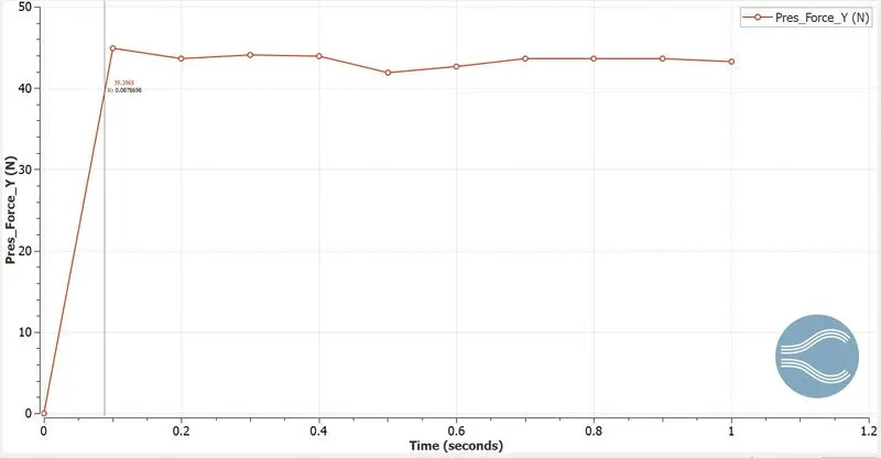
LIFT FORCE PLOT:

DRAG FORCE PLOT:

YPLUS PLOT:

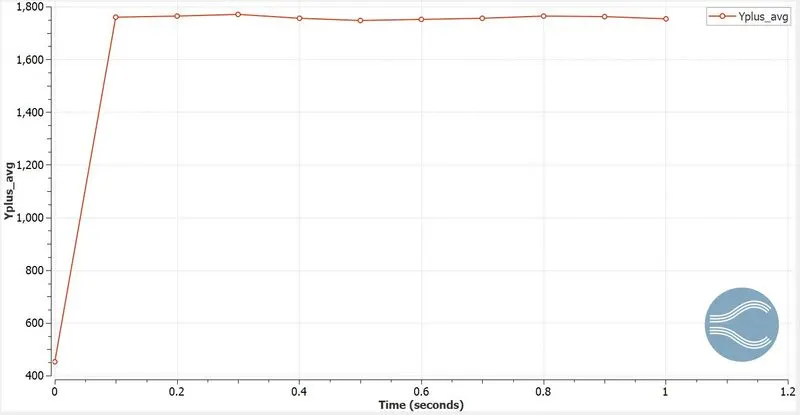
From this plot we can see that the yplus value is more than usual, the yplus value should be in the range between 300 to 400. But for this simulation, we have run this model using coarse mesh due to limited cell by license.

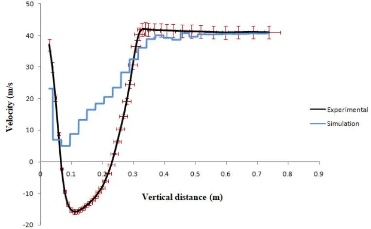
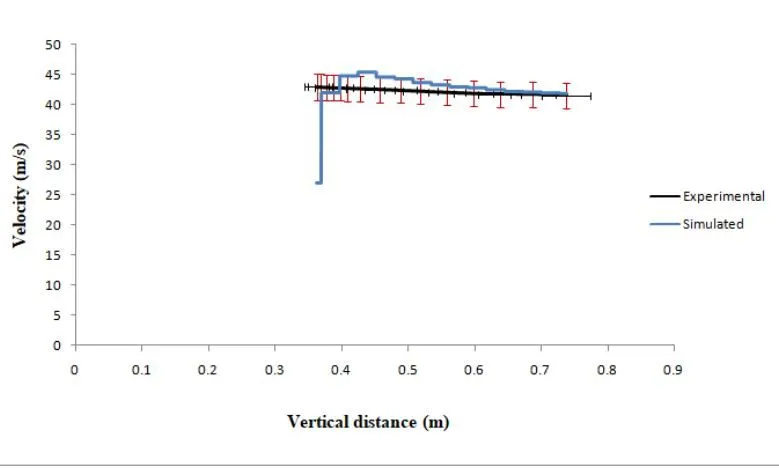
COMPARATIVE STUDY WITH EXPERIMENTAL ANALYSIS :

To analyze the obtained data with experimental results, we need to plot the line probes for different locations in the body w.r.t the velocity of the flow around it. This helps us to know the velocity at different locations on or above the body.

At x = -13mm and y = 0 mm at x = 37mm and y= 0 mm

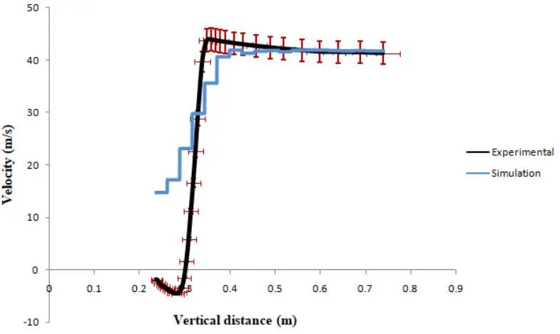
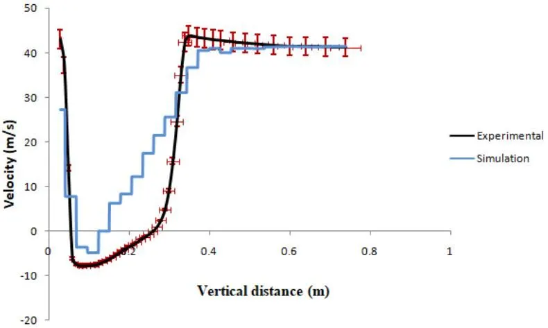
x = -63 mm and y = 0mm x = 87mm and y = 0mm

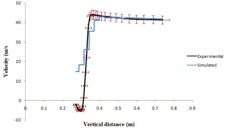
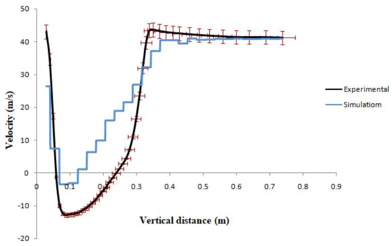
x = -113mm and y = 0mm x = 137mm and y = 0mm

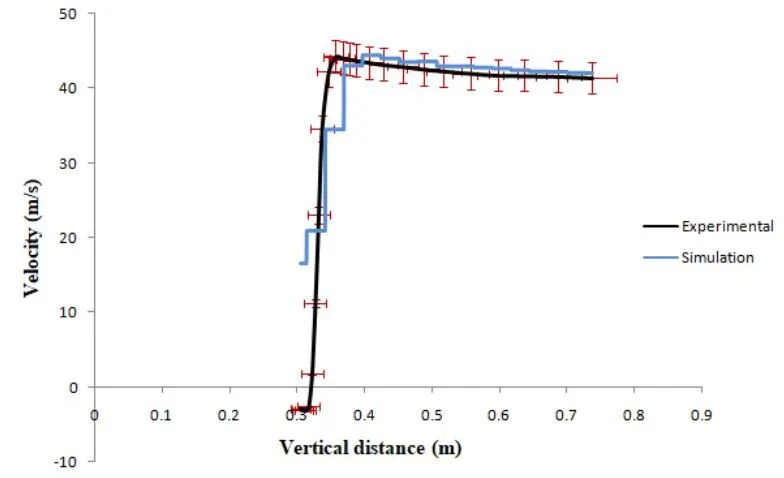
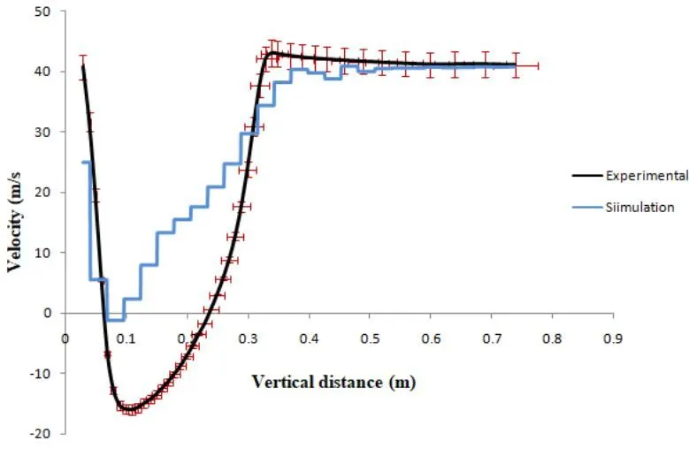
x = 187mm and y = 0mm at x = -263mm and y = 0mm

CONCLUSION:

• To calculate the coefficient of lift,

  `Cl=L/(1/2*rho*v^2*s)`

  `rho` denotes the density of air which is 1.225

  `v^2` denotes the velocity of air at the inlet is 40 m/s

  `s` denotes the surface area of the airfoil which is 0.112m^2

  `Cl = 43.5/(1/2*1.225*40^2*0.112)`

  `Cl = 0.396` 109.76

• To calculate the coefficient of drag,

  `Cd=D/(1/2*rho*v^2*s)`

  `rho` denotes the density of air which is 1.225

  `v^2` denotes the velocity of air at the inlet is 40 m/s

  `s` denotes the surface area of the airfoil which is 0.112m^2

  `Cd = 77.63/(1/2*1.225*40^2*0.112)`

  `Cd = 0.707`

• From this simulation, we understand the concept of box embedding.
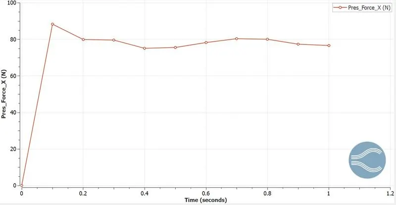
• When the Ahmed body is traveling at 40 m/s, 77.63 N of drag force is produced.
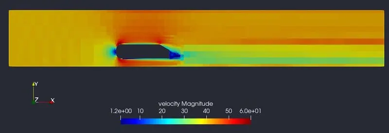
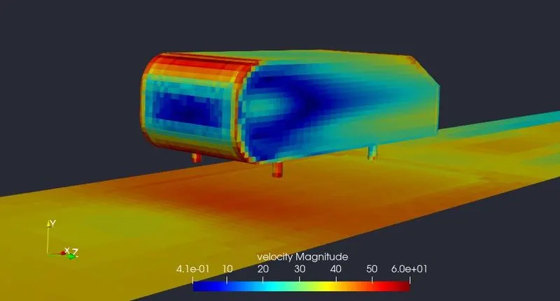
• We can also visualizes that vortex is been produced at the end of the Ahmed body.