Week 7: Shock tube simulation project

AIM:

• To simulate the flow in a shock tube to see the mass reaction of both N2 and O2 while the air enters from high pressure to low pressure.
• This simulation is used to understand the concept of flow flowing from high pressure to low pressure.

THEORY:

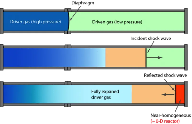
Bursting of the diaphragm results in the creation of shock waves. Compression waves propagate in the low-pressure section whereas expansion waves in the high pressure section. Shock waves get refracted back resulting in the mixing of the fluid.

PROCEDURE FOR SETTING UP THE SIMULATION CASE:

Importing Geometry & Diagnosis:

• Import the geometry in the STL file which is in the form of triangles.
• After importing run the diagnosis for checking the geometry for any problem in cad.
• Most important this that we need to check the normal also, the normal should be pointing towards the domain.

Case set-up :

• The application type is Timebase.
• A predefined air mixture is used.
• Using turbulent Prandtl number 0.9.
• Using turbulent Schmidt number 0.78.
• O2 and N2 are species of air.

Simulation Parameters:

• A transient-state solver is used.
• Starting time is 0s and the ending time is 0.5.
• The minimum time step is 1e-9s.
• The maximum time step is 1s.

Boundary Condition and Region Initialization:

• The high-pressure region, Low-pressure region, High-pressure 2D, Low-pressure 2D total four boundaries are used.
• In this simulation, we are going to the high-pressure region as the wall as well as the low-pressure region as a wall.
• Both 2D high pressure and low pressure are considered 2D.
• In region initialization, we are going to create two regions one as high pressure of about 600000.0 pa and low pressure of atmospheric pressure about 101325 pa.
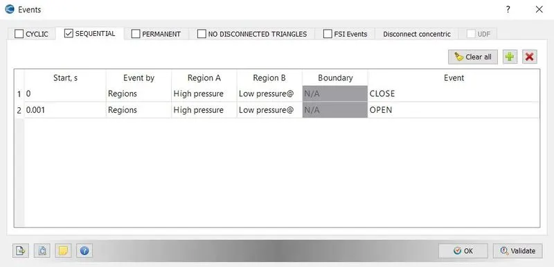
• Here we are going to use the event method to allow the flow from high pressure to low pressure after some time.

Physical Model:

• We are using RANS_K_EPS_RNG ( Re-Normalisation Group) turbulence model.

Grid Control:

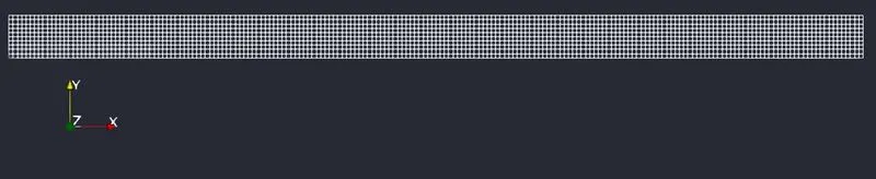
• In grid control, we will be defining the mesh size for the domain (0.002 m is the mesh size).
• Here we are using adaptive mesh refinement for accurate capture of flow physics.

Output and Post-processing:

• In the post-variable selection, we can select the output that we need for post-processing.
• In output files, we can set time intervals for writing the 3D output.
• We can also set time intervals for writing, restarting files.

Running Simulation:

• After finishing setting up the simulation case we need to export the input files in a folder.
• Now open the Cygwin terminal and navigate to the folder where you exported the input files.
• Now run the executable mpiexec.exe -n 2 converge.exe restricted.
• After finishing the simulation we need to convert the output file to paraview format.
• mpiexec.exe -n 2 post_convert_30_msmpi_64.exe command is used to convert the file as ParaView format.

RESULT:

MESH GENERATION:

MASS FRACTION OF N2:

MASS FRACTION OF O2:

ANIMATION OF MASS FRACTION N2:

ANIMATION OF MASS FRACTION O2:

ANIMATION OF VELOCITY CONTOUR:

ANIMATION OF PRESSURE CONTOUR:

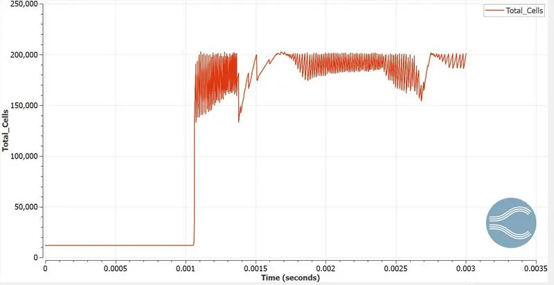
TOTAL CELL COUNT PLOT:

CONCLUSION:

• In the above analysis, flow through shock waves is simulated.
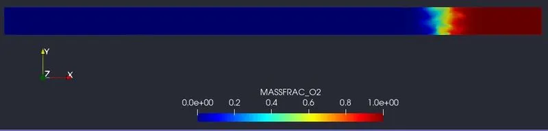
• The mixing is characterized by abrupt fluctuation in pressure, density, and velocity as can be observed from the plots.
• Cell count varies once the shock wave is created. The variation is primarily due to adptive mesh refinement and rupturing of the diaphragm.