Week 6: Conjugate Heat Transfer Simulation

AIM:

To simulate Conjugate heat transfer through the pipe using Super-cycling in converge software and to find the Y+ value as well as understanding the concept.

Theory:

CONJUGATE HEAT TRANSFER:

• CHT has a combination of both solid and fluid interactions.
• In CHT problems heat conduction takes place in the fluid domain only.
• We have many CHT applications eg, Heatsink, IC engine, etc.

SUPER-CYCLING METHOD:

• The super-Cycling method is used only for conduction or heat transfer-based problems.
• In this method, the fluid solver stops for some time and allowing the solid-state solver to catch up with the results.
• This method reduced the number of cycled and simulation times.

CALCULATION OF VELOCITY USING REYNOLDS NUMBER:

• `Re = (rho*V*D)/mu`.
• Re is Reynolds number which is 7000.
• `rho` is the density of air 1.225.
• V is the velocity, which is needed to find out.
• D is the diameter of the pipe.
• `mu` is the dynamic viscosity of air, which is `1.872*10e^-5``
• `7000 = (1.225*V*0.015)/(1.872*e^-5)`
• `V=(1.872*e^-5*7000)/(1.225*0.015)`
• `therefore V =7.1 (m)/(s)`

PROCEDURE FOR SETTING UP THE SIMULATION CASE:

Creating Geometry & Diagnosis:

• Create the geometry using the create option, select the cylinder in shape, and give geometry dimension.
• After importing run the diagnosis for checking the geometry for any problem in cad.
• Most important this that we need to check the normal also, the normal should be pointing towards the domain.

Case set-up :

• The application type is Timebase.
• A predefined air mixture is used.
• Using turbulent Prandtl number 0.9.
• Using turbulent Schmidt number 0.78.
• O2 and N2 are species of air.

Simulation Parameters:

• A transient-state solver is used.
• Starting time is 0s and the ending time is 0.5.
• The minimum time step is 1e-9s.
• The maximum time step is 1s.

Boundary Condition and Region Initialization:

• Inlet, Outlet, solid wall, sold side, and Intersection boundary wall total four boundaries are used.
• Inlet is considered as Inflow and has a velocity of about 7 m/s, in species we have air.
• The outlet is considered as Outflow and has a pressure of about 101325 pa and air as back-flow.
• The solid wall is considered a slip condition and has a heat flux of about -10000 W/m2.
• The solid sidewall is considered as a slip in numen condition.
• The intersection boundary is considered an intersection boundary.
• In region initialization, we are going to create two regions as solid region and fluid region in the boundary condition.
• Species in region initialization is also air.

Physical Model:

• We are using RANS_K_EPS_RNG ( Re-Normalisation Group) turbulence model.
• Here we are going to enable turbulence modeling which reduces the number of cycles and reduces the simulation time.

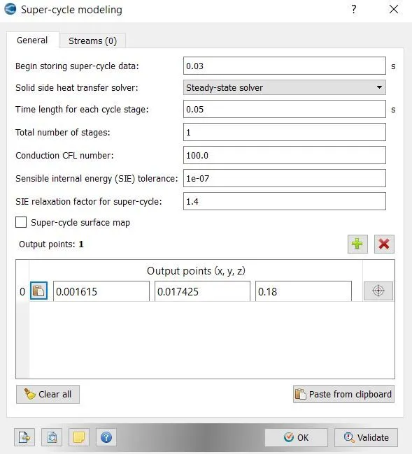
Grid Control:

• In grid control, we will be defining the mesh size for the domain (0.002 m is the mesh size).

Output and Post-processing:

• In the post-variable selection, we can select the output that we need for post-processing.
• In output files, we can set time intervals for writing the 3D output.
• We can also set time intervals for writing, restarting files.

Running Simulation:

• After finishing setting up the simulation case we need to export the input files in a folder.
• Now open the Cygwin terminal and navigate to the folder where you exported the input files.
• Now run the executable mpiexec.exe -n 2 converge.exe restricted.
• After finishing the simulation we need to convert the output file to paraview format.
• mpiexec.exe -n 2 post_convert_30_msmpi_64.exe command is used to convert the file as ParaView format.

RESULT:

GRID INDEPENDENCE STUDY:

MESH GENERATION:

Mesh Size 0.004:

Mesh Size 0.003:

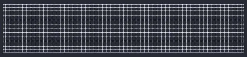
Mesh Size 0.0035:

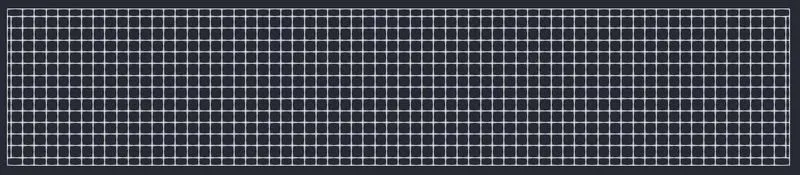
Mesh Size 0.0025:

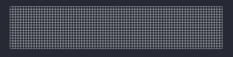
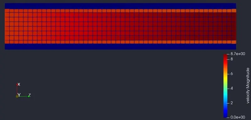
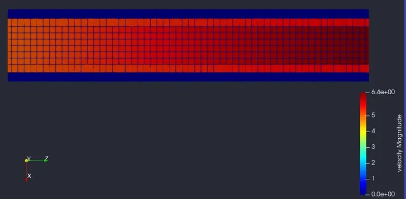
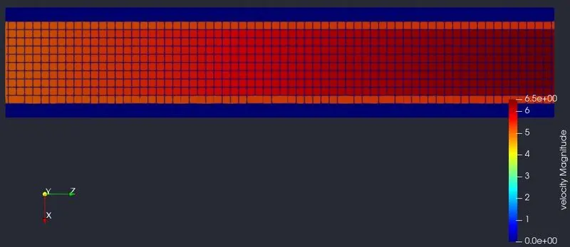
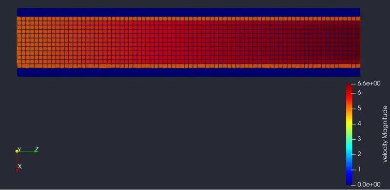
VELOCITY CONTOUR:

Mesh Size 0.004:

Mesh Size 0.003:

Mesh Size 0.0035:

Mesh Size 0.0025:

PRESSURE CONTOUR:

Mesh Size 0.004:

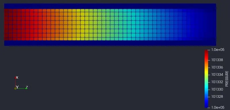
Mesh Size 0.003:

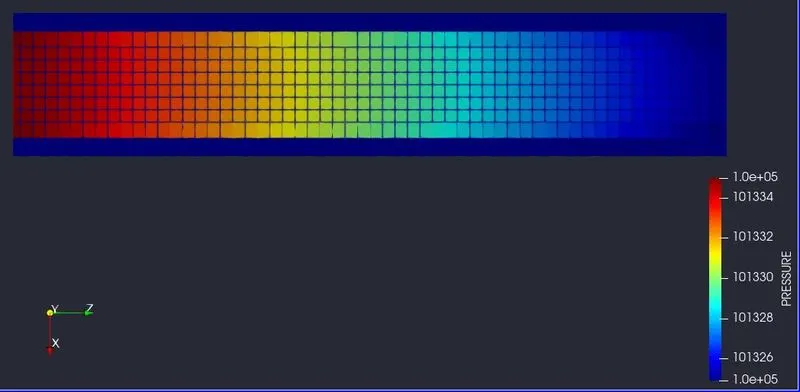
Mesh Size 0.0035:

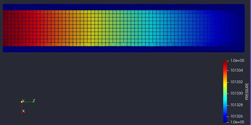
Mesh Size 0.0025:

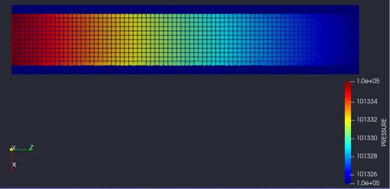
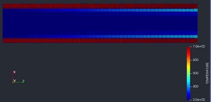
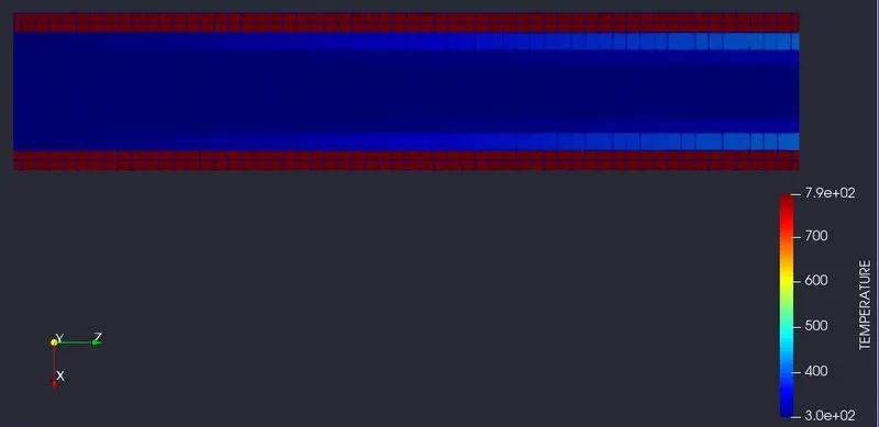
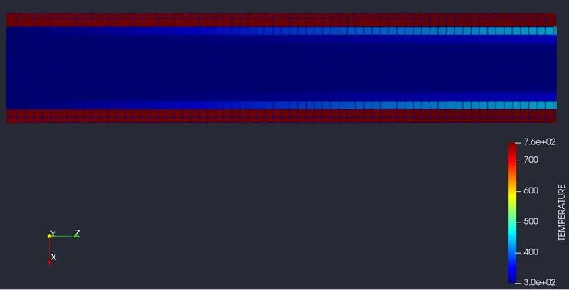
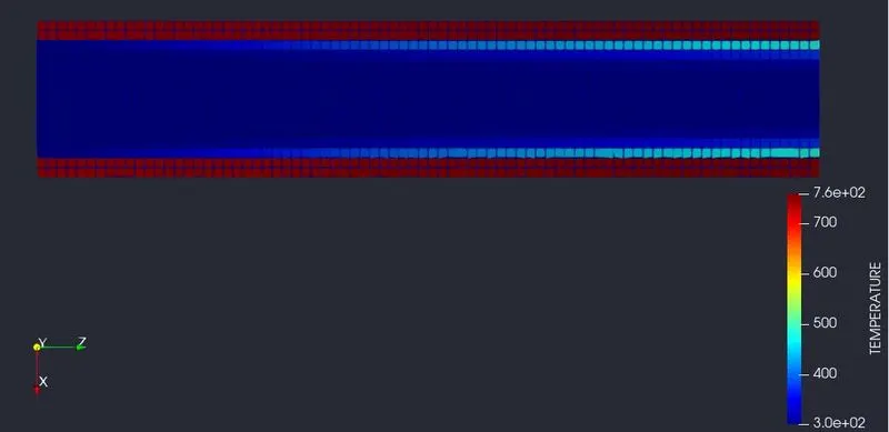
TEMPERATURE CONTOUR:

Mesh Size 0.004:

Mesh Size 0.003:

Mesh Size 0.0035:

Mesh Size 0.0025:

Y PLUS CONTOUR:

Mesh Size 0.004:

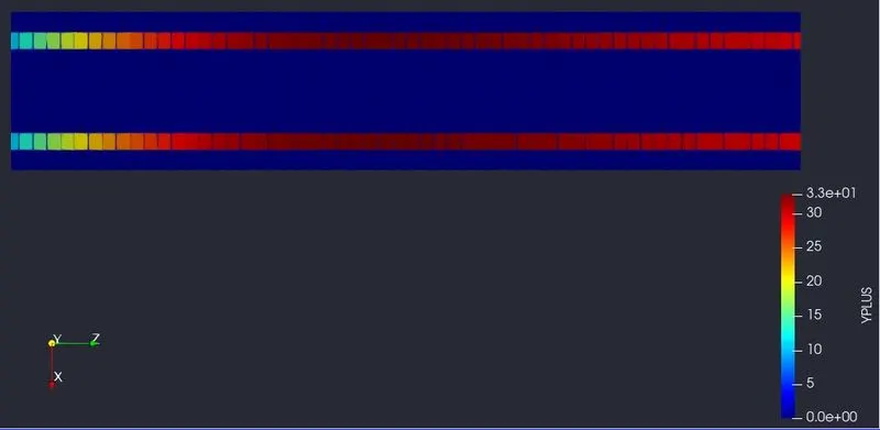
Mesh Size 0.003:

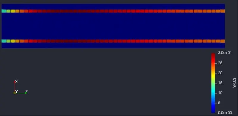
Mesh Size 0.0035:

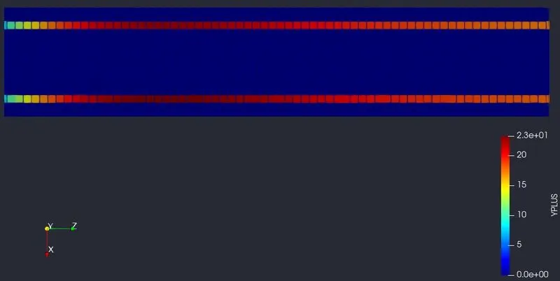
Mesh Size 0.0025:

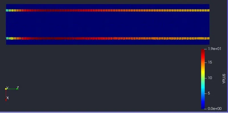
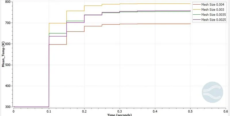
MEAN TEMPERATURE PLOT FOR DIFFERENT MESH SIZES:

ANIMATION FOR TEMPERATURE CONTOUR MESH SIZE 0.0025:

ANIMATION FOR VELOCITY CONTOUR MESH SIZE 0.0025:

Y PLUS VALUE FOR DIFFERENT MESH SIZES:

MESH SIZE	Y PLUS VALUE
0.004	`7.0e^02`
0.003	`3.0e^01`
0.0035	`2.3e^01`
0.0025	`1.9e^01`

SUPER-CYCLING METHOD:

We have simulated three different values for super cycling 0.01,0.02,0.03.

SUPER-CYCLING (s)	TIME TAKEN TO FINISH THE SIMULATION (s)
0.01	666.517079
0.02	677.039959
0.01	688.127531

CONCLUSION:

• From the Grid Independence study, we can come to know the Y plus value for different mesh.
• From the Y plus value, came to know that the mesh is fine and coarse, using this value we can say that the result is accurate or not.
• From the Super-Cycling method, we reduced the number of cycles as well as time for running simulation.