Week 5: Prandtl Meyer Shock problem

AIM:

• To simulate supersonic flow in duct having a sharp edge.
• To understand the concept of the adaptive mesh.

SHOCK WAVE:

A shock wave or shock is a type of propagating disturbance that moves faster than the local speed of sound in the medium. Like an ordinary wave, a shock wave carries energy and can propagate through a medium but is characterized by an abrupt, nearly discontinuous, change in pressure, temperature, and density of the medium. The shock wave is a strong pressure wave in any medium either in air or water. It is created by explosions, lightning, supersonic aircraft, and other phenomena that create violent changes in pressure.

BOUNDARY CONDITION FOR SHOCK WAVE:

Here the variables(pressure, temperature, Mach no., and velocity) are not available at the beginning. So nothing is specified at a supersonic outlet and all variables are extrapolated from the domain interior. Only the normal derivative of variables is specified as zero. So, Neumann boundary conditions are used in supersonic outlets.

PROCEDURE FOR SETTING UP THE SIMULATION CASE:

Importing Geometry & Diagnosis:

• Import the geometry in the STL file which is in the form of triangles.
• After importing run the diagnosis for checking the geometry for any problem in cad.
• Most important this that we need to check the normal also, the normal should be pointing towards the domain.

Case set-up :

• The application type is Timebase.
• A predefined air mixture is used.
• Using turbulent Prandtl number 0.9.
• Using turbulent Schmidt number 0.78.
• O2 and N2 are species of air.

Simulation Parameters:

• A steady-state solver is used.
• Starting cycle is 0 and the ending cycle is 15000.
• The initial time step is 1e-9s.
• The minimum time step is 1e-9s.
• The maximum time step is 1s.
• A pressure-based solver is used.
• The steady-state monitor is turned on, Mass flow rate is selected.
• The minimum number of cycles to execute for the steady-state monitor is 5000 cycles.

Boundary Condition and Region Initialization:

• Inlet, Outlet, Top and bottom wall, Front 2D and Back 2D total five boundaries are used.
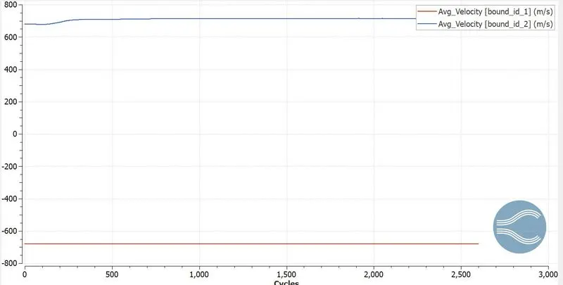
• Inlet is considered as Inflow and has a velocity of about 680 m/s, in species we have air.
• The outlet is considered as Outflow Numen boundary condition
• The top and bottom walls are considered as slip conditions.
• The front and Back portion is considered as 2D.
• In region initialization, we will a region where the fluid should flow and we assign this in the boundary condition.
• Species in region initialization is also air.

Physical Model:

• We are using RANS_K_EPS_RNG ( Re-Normalisation Group) turbulence model.

Grid Control:

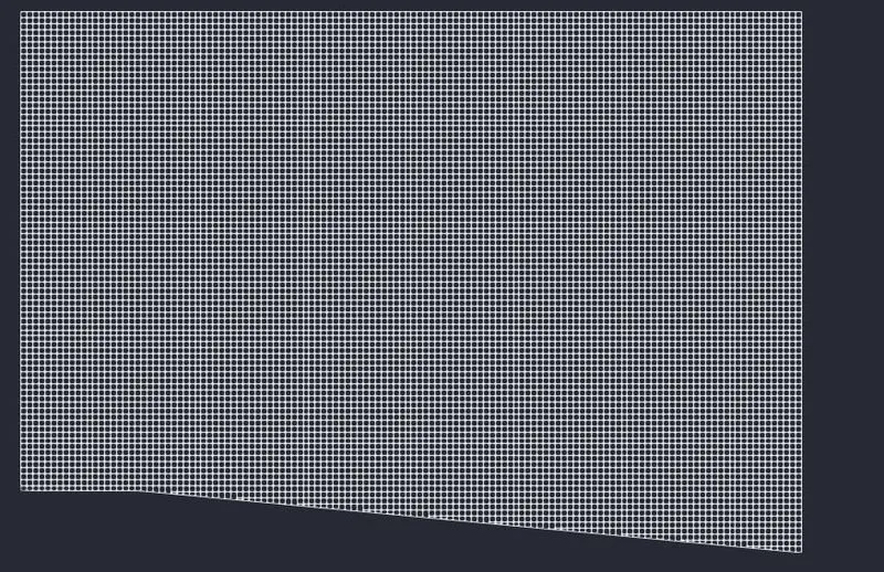
• In grid control, we will be defining the mesh size for the domain (0.002 m is the mesh size).
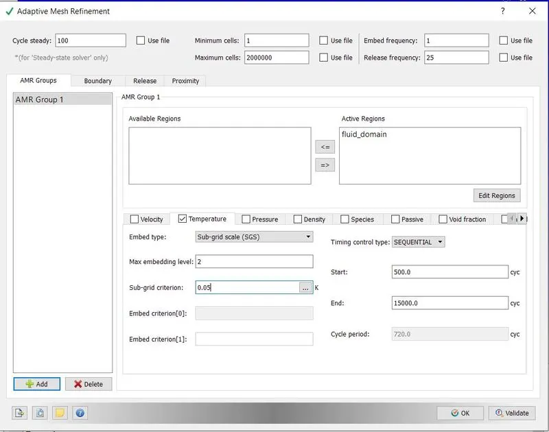
• Now we are going to enable Adaptive mesh refinement.
• In adaptive mesh embedding, we are going to mention the SGS parameter as 0.05.

Output and Post-processing:

• In the post-variable selection, we can select the output that we need for post-processing.
• In output files, we can set time intervals for writing the 3D output.
• We can also set time intervals for writing, restarting files.

Running Simulation:

• After finishing setting up the simulation case we need to export the input files in a folder.
• Now open the Cygwin terminal and navigate to the folder where you exported the input files.
• Now run the executable mpiexec.exe -n 2 converge.exe restricted.
• After finishing the simulation we need to convert the output file to paraview format.
• mpiexec.exe -n 2 post_convert_30_msmpi_64.exe command is used to convert the file as ParaView format.

RESULT:

Case 1 SGC parameter 0.05:

MESH GENERATION:

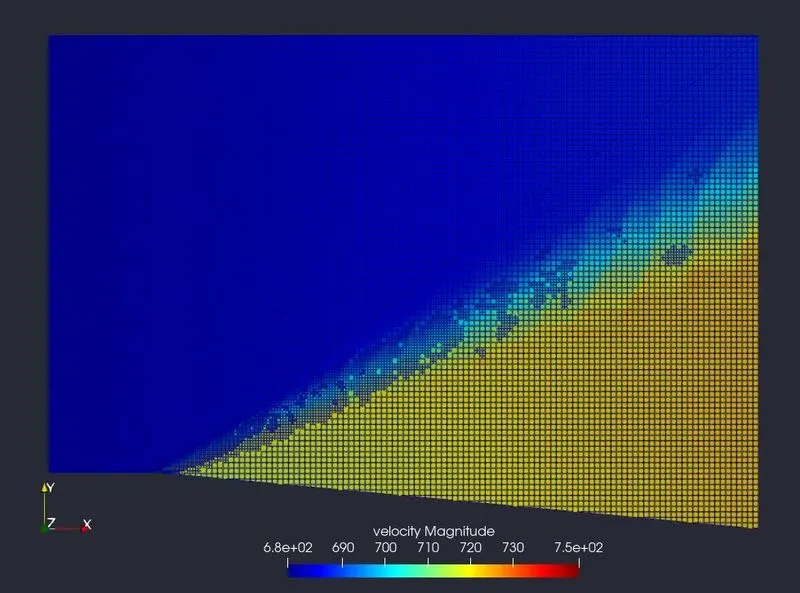
VELOCITY CONTOUR:

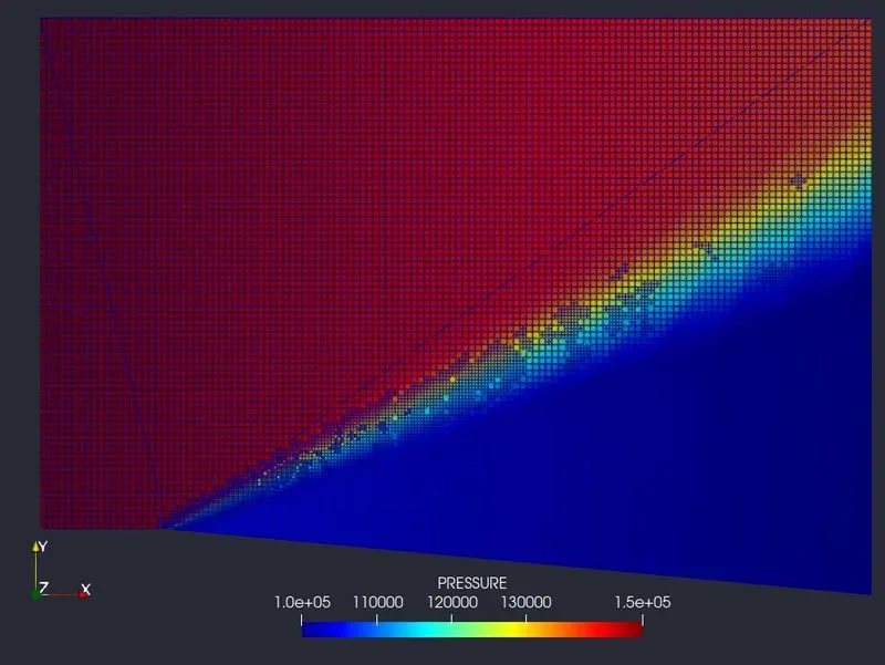
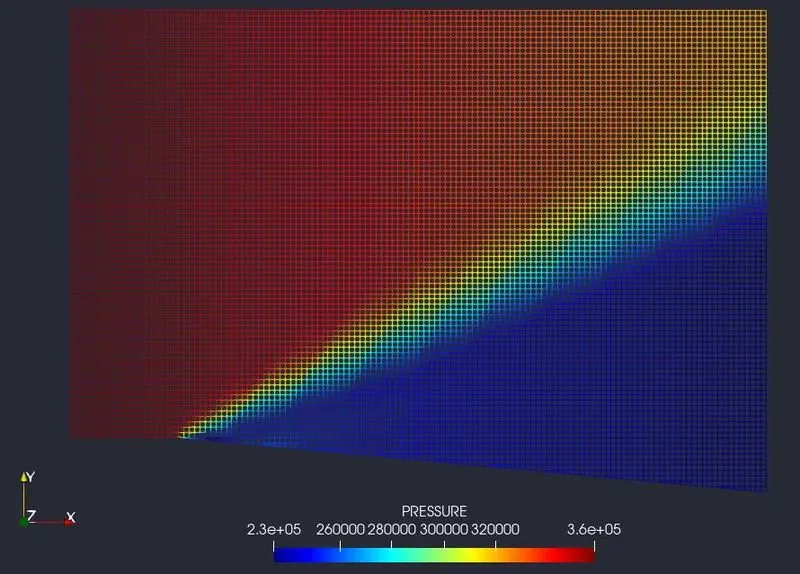
PRESSURE CONTOUR:

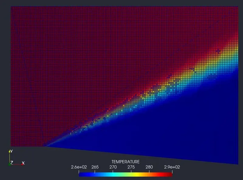
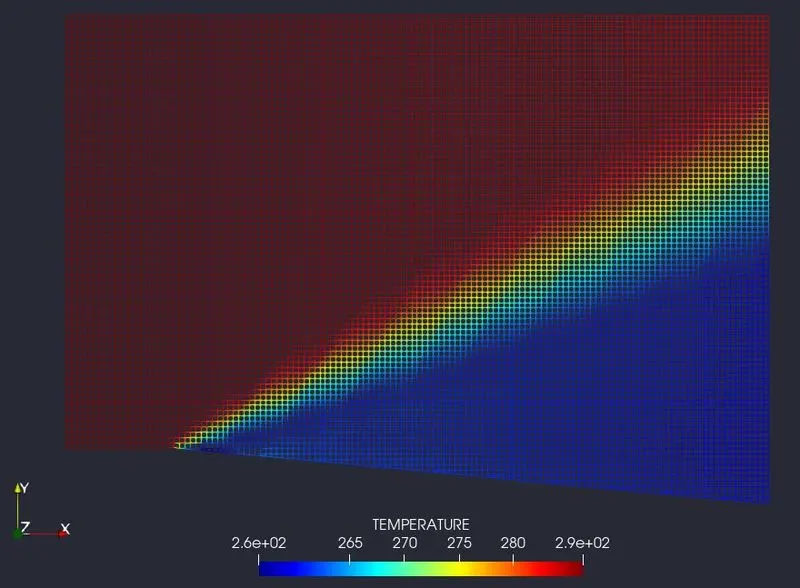
TEMPERATURE CONTOUR:

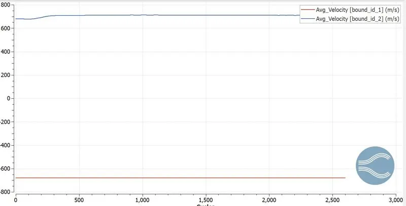
VELOCITY PLOT:

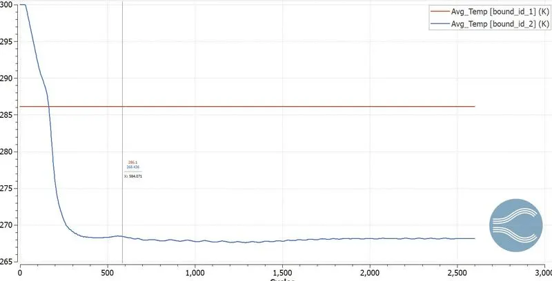
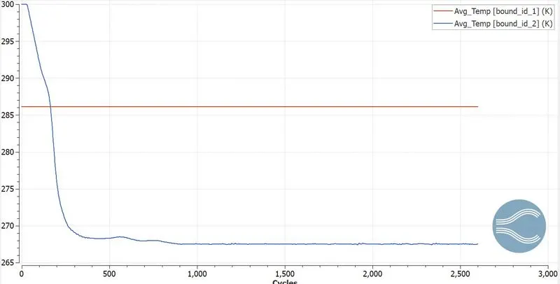
TEMPERATURE PLOT:

Case 1 SGC parameter 0.05:

MESH GENERATION:

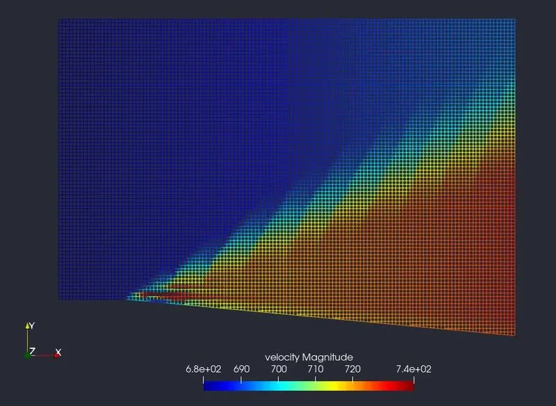
VELOCITY CONTOUR:

PRESSURE CONTOUR:

TEMPERATURE CONTOUR:

VELOCITY PLOT:

TEMPERATURE CONTOUR:

ANIMATION:

VELOCITY CONTOUR:

PRESSURE CONTOUR:

CONCLUSION:

• In supersonic flow, the Prandtl-Meyer expansion fan is clearly visible and the mesh refinement is also visible in the shock region.
• As the SGS parameter decreases, the total cell count increases, and the mesh refinement area spread from the sharp edge to the outlet boundary. If the SGS parameter increases, the mesh refinement area is very small and it doesn't spread to the outer boundary.