Week 11: FSAE Car Project

AIM:

• To simulate flow over an FSAE car to find out the drag force and downward force.
• There are two cases of track one track has lots of turns and another is the straight track.
• To compare the drag and downforce of two cases.

THEORY:

Formula SAE is a student design competition organized by SAE International (previously known as the Society of Automotive Engineers, SAE). The competition was started in 1980 by the SAE student branch at the University of Texas at Austin after a prior asphalt racing competition proved to be unsustainable.

DOWNFORCE:

Downforce is a downwards lift force created by the aerodynamic features of a vehicle. If the vehicle is a car, the purpose of downforce is to allow the car to travel faster by increasing the vertical force on the tires, thus creating more grip. If the vehicle is a fixed-wing aircraft, the purpose of the downforce on the horizontal stabilizer is to maintain longitudinal stability and allow the pilot to control the aircraft in pitch.

PROCEDURE TO SET UP THE CASE:

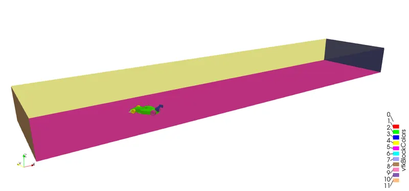
Importing Geometry, Creating Virtual Wind Tunnel & Diagnosis:

• Import the geometry in the STL file which is in the form of triangles.
• After importing run the diagnosis for checking the geometry for any problem in cad, then delete the overlapping edges and non-manifold edges by using the diagnosis tool.
• Here, in this case, we have two cases one is a straight track and another case has lots of turns in track, so the domain size varies for these two cases.
• Most important this that we need to check the normal also, the normal should be pointing towards the domain.

Case set-up :

• The application type is Timebase.
• A predefined air mixture is used.
• Using turbulent Prandtl number 0.9.
• Using turbulent Schmidt number 0.78.
• O2 and N2 are species of air.

Simulation Parameters:

• A transient-state solver is used.
• End time can be calculated, End time = length of the domain/velocity.
• We get End time = 0.1827, which is the one cycle.
• We are going to run the simulation 4 cycle then `2*2.6 approx 5.2s`
• The minimum time step is 1e-9s.
• The maximum time step is 1s.

Boundary Condition and Region Initialization:

• The Inlet, Outlet, Top and sidewall, Car parts, Bottom wall, are boundaries.
• Inlet and velocity inlet and velocity as 20.11 m/s and species as air.
• Outlet as pressure outlet of 101325 pa and backflow species as air.
• The top and sidewall are considered as Symmetry.
• The bottom wall is considered a wall as the law of the wall.
• All car parts are considered a wall and the law of wall condition are provided.
• In Region & Initialization, we create a region for fluid flow and set the velocity as 20.11m/s.

Physical Model:

• We are using the k−ωSST turbulence model, which has automatic wall treatment.

Grid Control:

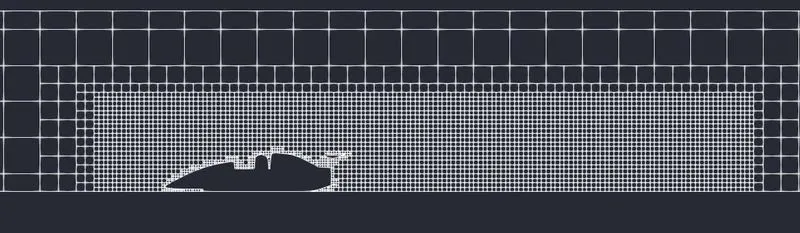
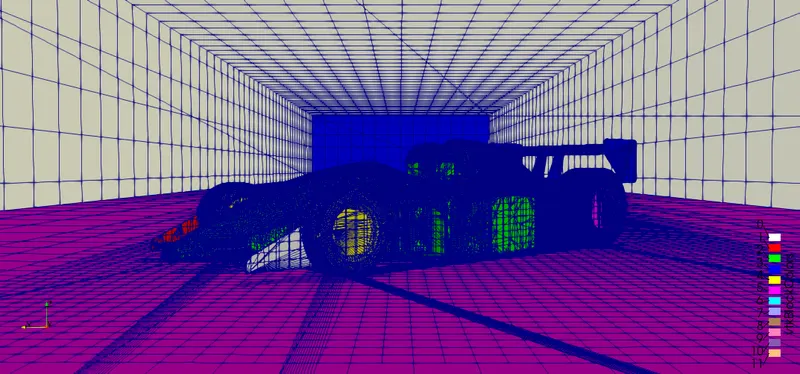
• In grid control, we will be defining the mesh size for the domain (0.5 m is the mesh size).
• Here we are using fixed embedding to refine the mesh to capture the flow physics.
• In fixed embedding, we are using the box method which will create a boundary over the test object.
• If you see that the boundary will have well-refined mesh but outside the mesh well be coarse mesh.

Output and Post-processing:

• In the post-variable selection, we can select the output that we need for post-processing.
• In output files, we can set time intervals for writing the 3D output.
• We can also set time intervals for writing, restarting files.

Running Simulation:

• After finishing setting up the simulation case we need to export the input files in a folder.
• Now open the Cygwin terminal and navigate to the folder where you exported the input files.
• Now run the executable mpiexec.exe -n 2 converge.exe restricted.
• After finishing the simulation we need to convert the output file to paraview format.
• mpiexec.exe -n 2 post_convert_30_msmpi_64.exe command is used to convert the file as ParaView format.

RESULTS:

CASE 1

MESH GENERATION:

VELOCITY CONTOUR:

VELOCITY OVER THE BODY:

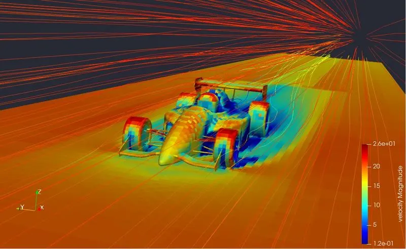
VELOCITY STREAMLINES:

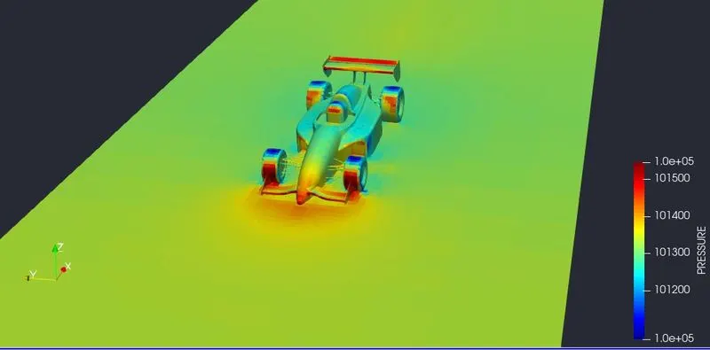
PRESSURE CONTOUR:

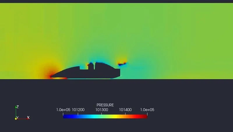
PRESSURE OVER THE BODY:

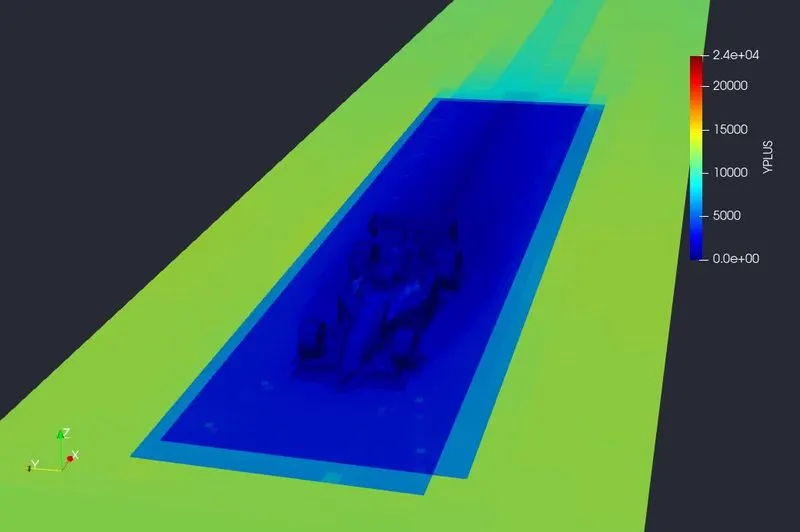
YPLUS :

YPLUS PLOT FOR ALL CAR PARTS:

DRAG FORCE PLOT FOR CAR PARTS:

DOWNWARD FORCE PLOT FOR ALL CARS PARTS:

CASE 2 LOTS OF TURNS IN TRACK:

MESH GENERATION:

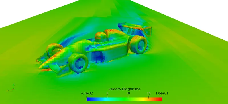
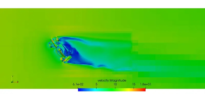
VELOCITY OVER THE CAR:

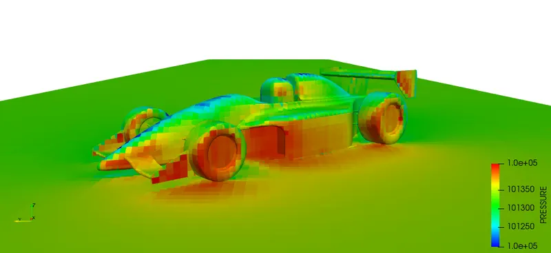
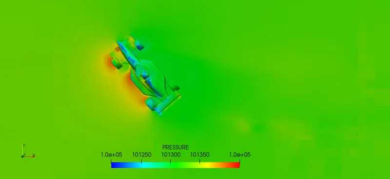
PRESSURE OVER THE CAR:

DRAG FORCE PLOT FOR ALL CAR PARTS:

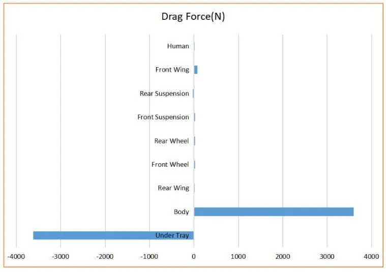
DOWNWARD FORCE FOR ALL CAR PARTS:

CONCLUSION:

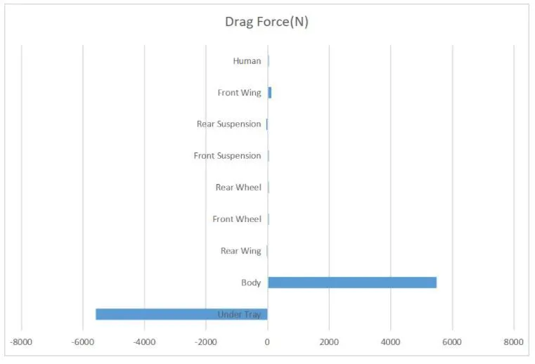
After analyzing the data and the result, it was observed that wheels or tires generated a portion of overall drag. To reduce drag on tires, wheels can be covered to make it more aerodynamic. Due to regulation, full covering might not be allowed, but if partial bodywork is permitted, placing converging fairing behind the wheels provides maximum benefit.

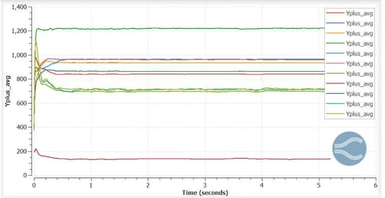
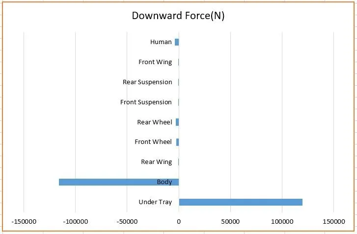
The flow over the rear wing as seen that it creates lift force over the corners by seeing the velocity profiles. This is because of the generation vortices and the airfoil in the car wing usually have a low aspect ratio and in turn, it creates the drag behind the body and also reduces the angle of attack of free stream air. To improve the lift is to increase airfoil thickness and also increase the height of the endplate. The Y plus is uniform throughout the body. The forces on the suspension links are very low and there is a need for a change of suspension links.