Week 3: Flow over a backward facing step

AIM:

• To simulate backward-facing step for different mesh size 2e-3,1.5e-3 & 1.2e-3.
• To visualize velocity & pressure contour for different mesh sizes.
• To understand the turbulent flow in the backward-facing step.

THEORY OF BACKWARD-FACING STEP:

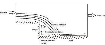
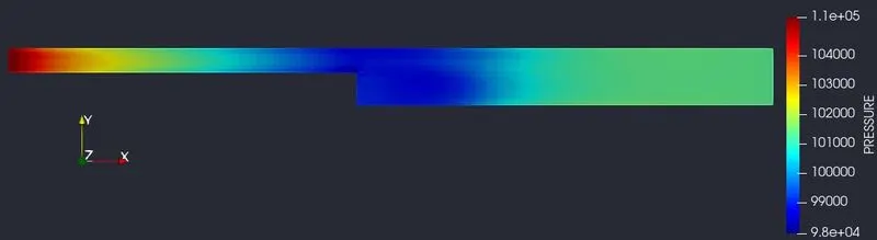
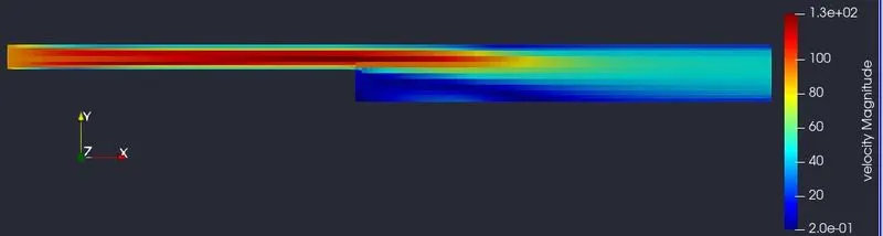
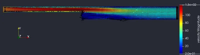
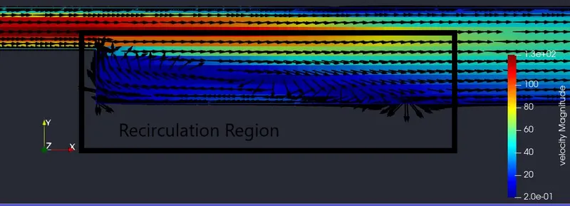
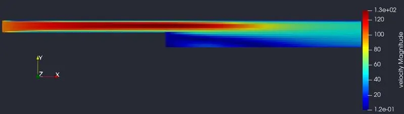
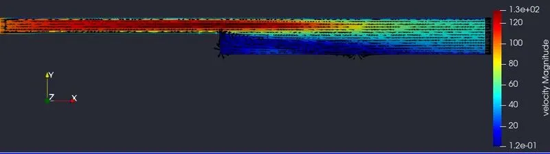
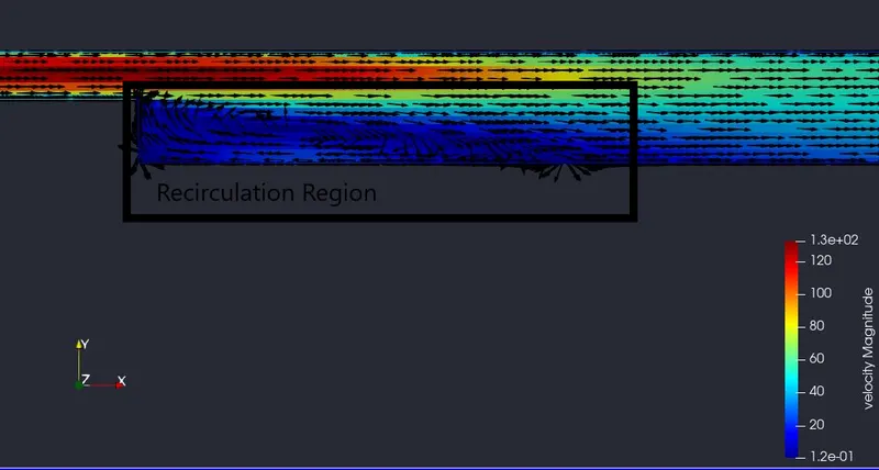
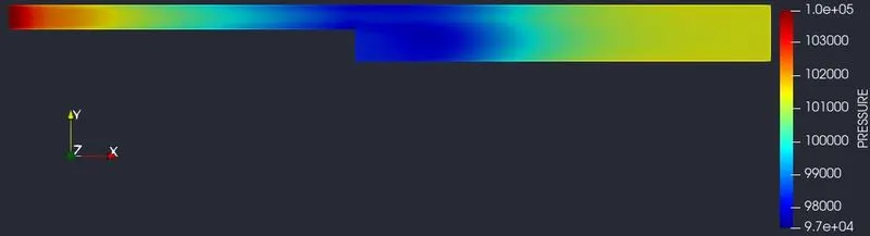
In this simulation, the flow is coming from the left side & suddenly a step is introduced in the domain then the is separated and the recirculation zone is formed. At the step region, the pressure value decreases and the velocity suddenly increases so the recirculation zone is formed. The flow from the inlet was laminar and it changes as turbulent when it reaches the step due to the flow separation which causes the recirculation of flow. After some time the flow is reattached at the bottom wall.

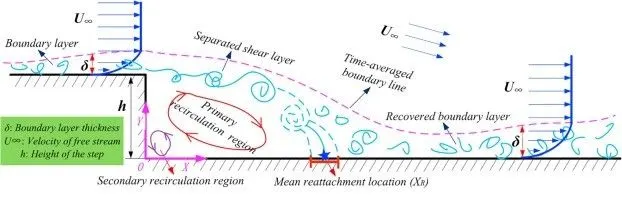
The above image is an example that our results will be also like this. When the flow enters into the domain it is in laminar condition while it comes to the step region the flow separates and the flow also becomes turbulent which causing the recirculation region. After some time this recirculated air is attached to the bottom wall and the turbulent flow is now turned into the laminar flow. The recirculation region is below the separated shear layer. This simulation has both laminar and turbulent flow.

This backward face simulation is the best case to test validate your code or turbulence model. The separation and reattachment of flow are an experiment in much practical application, Flow over an airfoil is one of the best practical applications.

PROCEDURE FOR SETTING UP THE SIMULATION CASE:

Importing Geometry & Diagnosis:

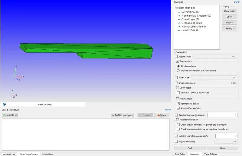
• Import the geometry in the STL file which is in the form of triangles.
• After importing run the diagnosis for checking the geometry for any problem in cad.
• Most important this that we need to check the normal also, the normal should be pointing towards the domain.

Case set-up :

• The application type is Timebase.
• A predefined air mixture is used.
• Using turbulent Prandtl number 0.9.
• Using turbulent Schmidt number 0.78.
• O2 and N2 are species of air.

Simulation Parameters:

• A steady-state solver is used.
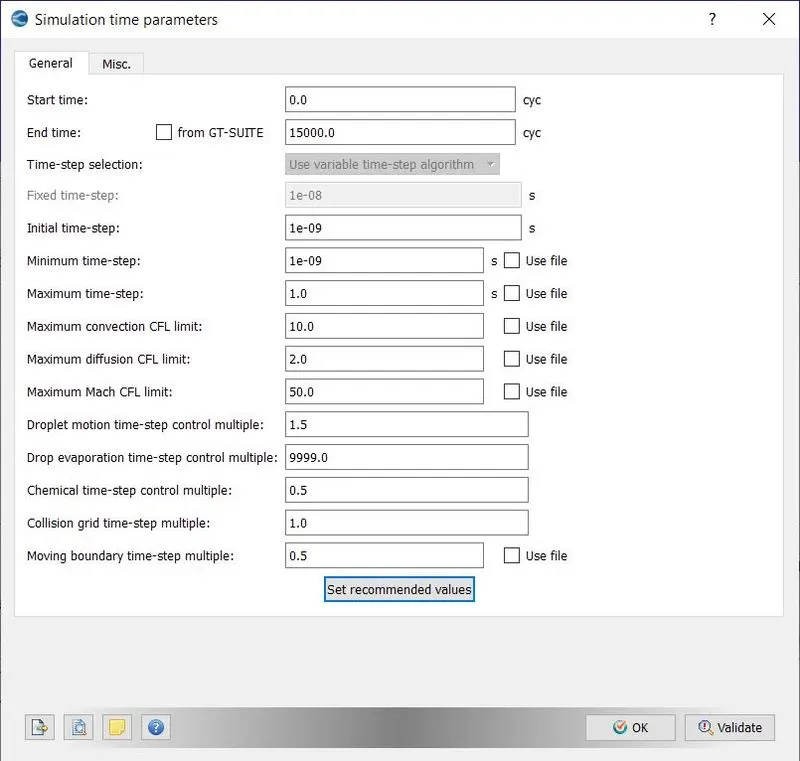
• Starting cycle is 0 and the ending cycle is 15000.
• The initial time step is 1e-9s.
• The minimum time step is 1e-9s.
• The maximum time step is 1s.
• A pressure-based solver is used.
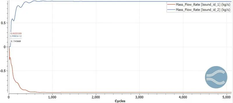
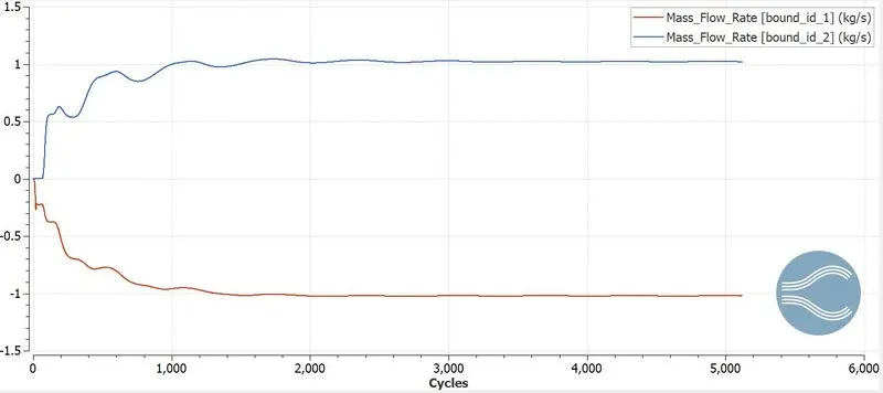
• The steady-state monitor is turned on, Mass flow rate is selected.
• The minimum number of cycles to execute for the steady-state monitor is 5000 cycles.

Boundary Condition and Region Initialization:

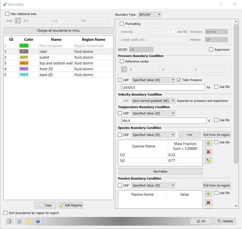
• Inlet, Outlet, Top and bottom wall, Front 2D and Back 2D total five boundaries are used.
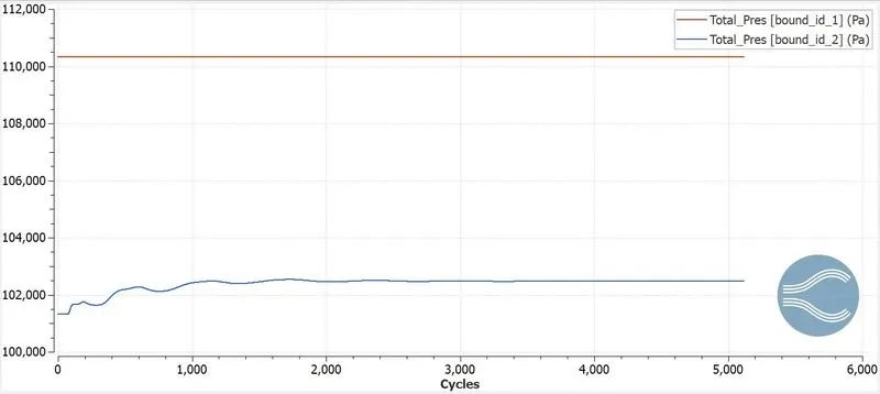
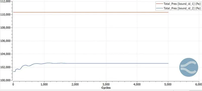
• Inlet is considered as Inflow and has a pressure of about 110325 pa, in species we have air.
• The outlet is considered as Outflow and has a pressure of about 101325 pa, if we have backflow then we have air as species.
• The top and bottom walls are considered as No-slip conditions.
• The front and Back portion is considered as 2D.
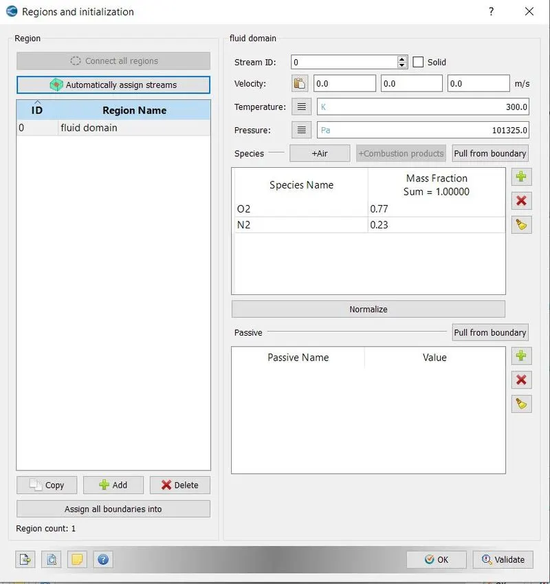
• In region initialization, we will a region where the fluid should flow and we assign this in the boundary condition.
• Species in region initialization is also air.

Physical Model:

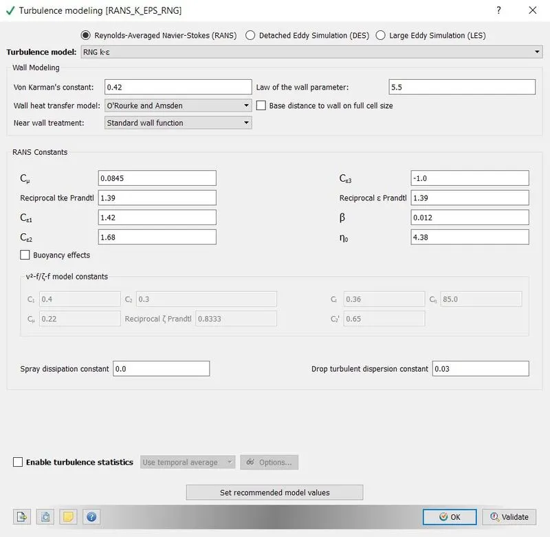
• We are using RANS_K_EPS_RNG ( Re-Normalisation Group) turbulence model.

Grid Control:

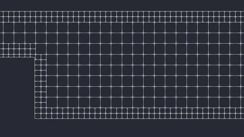
• In grid control, we will be defining the mesh size for the domain.
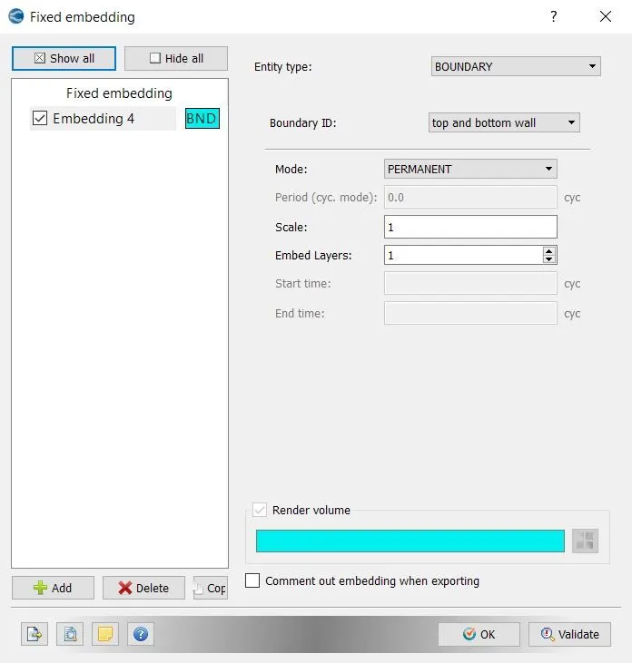
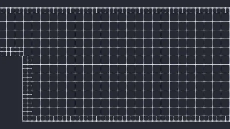
• Now we are going to enable Fixed embedding.
• In fixed embedding, we are going the define where the mesh is to be refined so we can capture the flow properties very accurately without decreasing the mesh size.

Output and Post-processing:

• In the post-variable selection, we can select the output that we need for post-processing.
• In output files, we can set time intervals for writing the 3D output.
• We can also set time intervals for writing, restarting files.

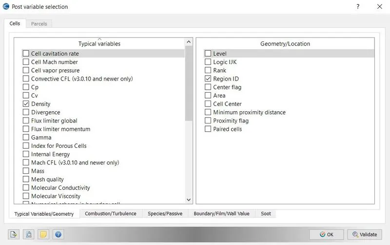
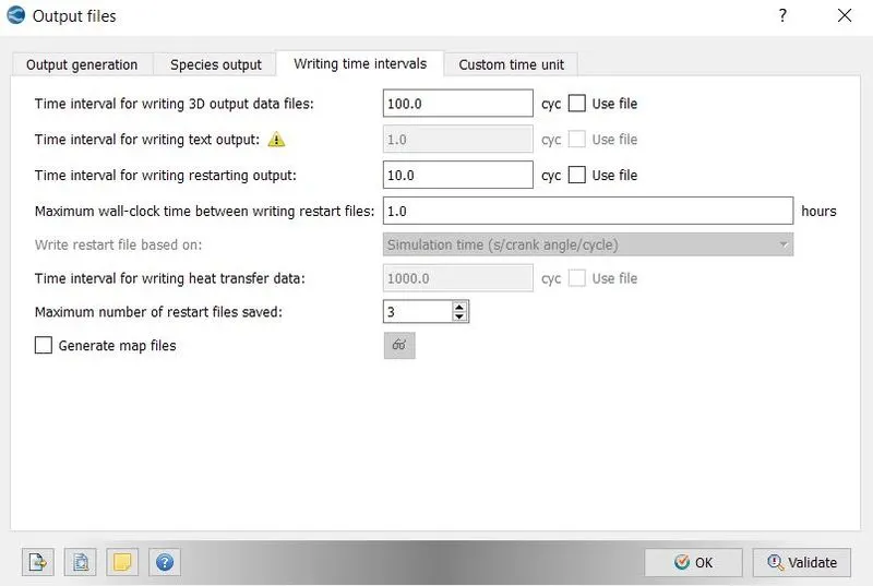
• After finishing setting up the simulation case we need to export the input files in a folder.
• Now open the Cygwin terminal and navigate to the folder where you exported the input files.
• Now run the executable mpiexec.exe -n 2 converge.exe restricted.
• After finishing the simulation we need to convert the output file to paraview format.
• mpiexec.exe -n 2 post_convert_30_msmpi_64.exe command is used to convert the file as ParaView format.

RESULTS:

Case 1 mesh size 2e-3:

MESH GENERATION:

PRESSURE CONTOUR:

VELOCITY CONTOUR:

VECTOR PLOT:

MASS FLOW RATE:

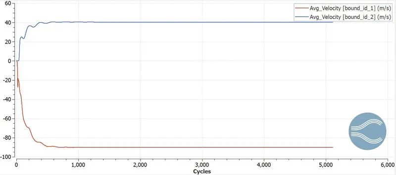
AVERAGE VELOCITY PLOT:

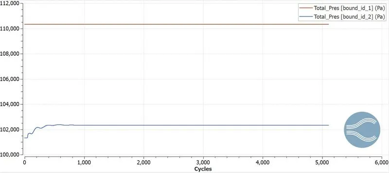
TOTAL PRESSURE PLOT:

VELOCITY CONTOUR ANIMATION:

PRESSURE CONTOUR ANNIMATION:

Case 2 mesh size 1.5e-3:

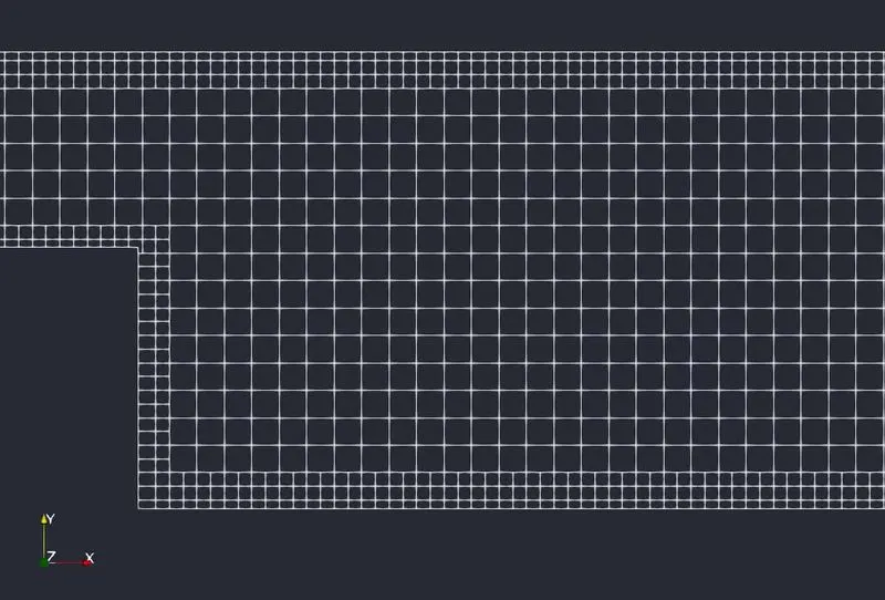
MESH GENERATION:

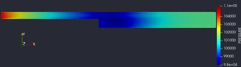
PRESSURE CONTOUR:

VELOCITY CONTOUR:

VECTOR PLOT:

MASS FLOW RATE:

TOTAL PRESSURE PLOT:

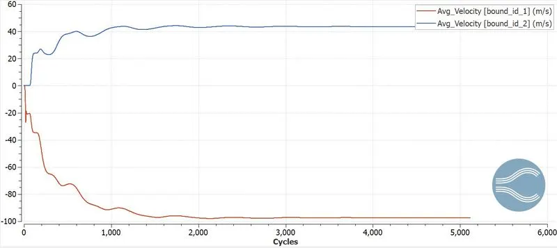
AVERAGE VELOCITY PLOT:

VELOCITY CONTOUR ANIMATION:

PRESSURE CONTOUR ANIMATION:

Case 3 mesh size 1.2e-3:

PRESSURE CONTOUR:

VELOCITY CONTOUR:

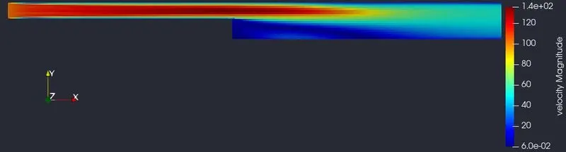
VECTOR PLOT:

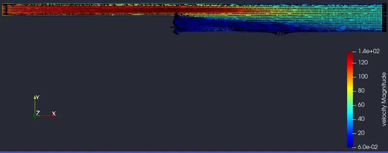
MASS FLOW RATE:

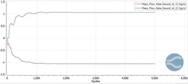
AVERAGE VELOCITY PLOT:

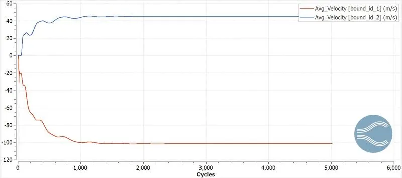
TOTAL PRESSURE PLOT:

VELOCITY CONTOUR ANIMATION:

PRESSURE CONTOUR ANIMATION:

CONCLUSION:

• While decreasing the mesh size we can see that the time for solving the problem is also increased and the results are also very accurate.
• We can compare mesh size 2e-3 and mesh size 1.2e-3 the results in the mesh size 2e-3 are inaccurate but the results in mesh 1.2e-3 are accurate.
• We understand the physics of the backward-facing step with different mesh size.