Week 7 - Simulation of a 1D Super-sonic nozzle flow simulation using Macormack Method

AIM:

To simulate 1D Super-sonic nozzle flow simulation using Macormack Method using Matlab code.

INTRODUCTION:

Description:

In this problem, we are going to see isentropic flow through a convergent-divergent nozzle. The flow from the inlet will be subsonic and as it comes to the throat section of the nozzle where the flow velocity will be equal to Mach 1 and the flow at the outlet will be supersonic.

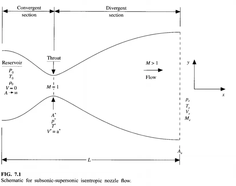
Governing Equation:

The governing continuity, momentum and energy equations in terms of non dimensional variables for this quasi one dimensional steady and isentropic flow can be expressed respectively as:

Non-Conservative Form:

• Continuity Equation:

`(delrho')/(delt') = -rho'((delV')/(delx')) - rho'V'((del(ln A'))/(delx')) - V'((delrho')/(delx'))`

• Momentum Equation:

`(delV')/(delt') = -V'((delV')/(delx')) -(1/gamma)((delT')/(delx') + (T')/(rho')((delrho')/(delx')))`

• Energy Equation:

`(delT')/(delt') = -V'((delT')/(delx')) - (gamma -1)T'[(delV')/(delx') + V'(del(lnA'))/(delx')]`

Conservative Form:

• Continuity Equation:

`(del(rho'A'))/(delt') + (del(rho'A'V'))/(delx') = 0`

• Momentum Equation:

`(del(rho'A'V'))/(delt') + (del[rho'A'(V')^2 +(1/gamma)rho'A'])/(delx') = (1/gamma)rho'((delA')/(delx'))`

• Energy Equation:

`(del[rho'((e')/(gamma-1) + (gamma/2)(V')^2)A'])/(delt') + (del[rho'((e')/(gamma-1) + (gamma/2)(V')^2)V'A' + rho'A'V'])/(delx') = 0`

Macormack Method:

This method has five steps,

let as consider f(x) is an equation to solve,

• Initial condition:

Before calculation, the initial value for velocity, temperature, and pressure should be determined.

• Predictor step condition:

`((delf)/(dt))_p = (f(i+1) - f(i))/(Deltax)`

• Solution Update:

`f_p = f_(Initial) + ((delf)/(delt))_p * Deltat`

`f_p`= values calculated after the predictor step

`f_(Initial)`= Initial Values

`Deltat`= time step size

• Corrector step condition:

`((delf_p)/(dt))_c = (f(i) - f(i-1))/(Deltax)`

`((delf)/(dt))_(avg) = 0.5(((delf)/(dt))_p +((delf_p)/(dt))_c )`

• Final Solution Update:

`f_(sol) = f_(Initial) + ((delf)/(delt))_(avg) * Deltat`

`f_(sol)`= Final solution for the values of first time step

MATLAB CODE:

Main code:

This is the main code for calling the functions:

close all
clear all
clc

% Input values
n = 31;
x = linspace(0,3,n);
dx = x(2)-x(1);
gamma = 1.4
c = 0.5; % Courant Number

% Time steps
nt = 1000;
dt = 0.0001;

% Function for Non-Conservative form
[mass_flow_rate, pressure, mach_number,rho,t,v,rho_old,t_old,v_old,rho_throat,t_throat,v_throat,a,throat,mass_flow_rate_throat,pressure_throat,mach_number_throat] = Non_conservative_form(x,dx,gamma,nt,c,n)

% Function for Conservative form
[mass_flow_rate_C, pressure_C, mach_number_C,  rho_C, v_C, t_C, rho_throat_C, v_throat_C, t_throat_C, mass_flow_rate_throat_C, pressure_throat_C, mach_number_throat_C] = Conservative_form(x, dx, n, gamma, nt, c)

Background of Code:

• Code is started with clear all, close all, and clc to enable a fresh start without the manipulation of previous values.
• Input parameters are assigned for the variables x, dx, n, gamma, nt and C.
• Non-Conservative and Conservative forms are created as separate functions with the necessary inputs

Non-Conservative Function Code:

This code contains the governing equations to solve the problem:

function [mass_flow_rate, pressure, mach_number,rho,t,v,rho_old,t_old,v_old,rho_throat,t_throat,v_throat,a,throat,mass_flow_rate_throat,pressure_throat,mach_number_throat] = Non_conservative_form(x,dx,gamma,nt,c,n)

% Calculate initial profile
rho = 1-0.3146*x; % Density
t   = 1-0.2314*x; % Temperature
v   = (0.1+1.09*x).*t.^0.5; % Velocity
a   = 1+2.2*(x-1.5).^2; %Area
throat = find(a==1); % Throat section

for k=1:nt
    dt = min(c.*dx./(sqrt(t) + v)) 
    dt = 0.01;
    rho_old = rho;
    v_old = v;
    t_old = t;
    
    % Predictor step
  drho_dt_p =0; 
  dv_dt_p=0;
  dt_dt_p=0;
    
    for j = 2:n-1
        % Continuity Equation
        %drho_dt_p = -rhodv_dx-rhovdloga_dx-vdrho_dx main equation
        % Sepearting the terms for easy debugging
        dv_dx    =  (v(j+1)-v(j))/dx;
        dloga_dx =  (log(a(j+1))-log(a(j)))/dx;
        drho_dx  =  (rho(j+1)-rho(j))/dx;
        dt_dx    =  (t(j+1)-t(j))/dx;
        
        drho_dt_p(j) = -(rho(j)*dv_dx) - (rho(j)*v(j)*dloga_dx) - (v(j)*drho_dx);
        
        % Momentum Equation
        dv_dt_p(j) = -(v(j)*dv_dx) - (1/gamma)*((dt_dx) + (t(j)/rho(j)*drho_dx));
        
        % Energy Equation
        dt_dt_p(j) = -(v(j)*dt_dx) - ((gamma-1)*t(j))*((dv_dx) + (v(j)*dloga_dx));
        % Solution Update
        rho(j) = rho(j)+drho_dt_p(j)*dt;
        v(j)   = v(j)+dv_dt_p(j)*dt;
        t(j)   = t(j)+dt_dt_p(j)*dt;
        
    end
    % Corrector method
      drho_dt_c =0; 
  dv_dt_c=0;
  dt_dt_c=0;
    for j = 2:n-1
        % Continuity Equation
        %drho_dt_c = -rhodv_dx-rhovdloga_dx-vdrho_dx main equation
        % Sepearting the terms for easy debugging
        dv_dx    =  (v(j)-v(j-1))/dx;
        dloga_dx =  (log(a(j))-log(a(j-1)))/dx;
        drho_dx  =  (rho(j)-rho(j-1))/dx;
        dt_dx    =  (t(j)-t(j-1))/dx;
        
        drho_dt_c(j) = -(rho(j)*dv_dx) - (rho(j)*v(j)*dloga_dx) - (v(j)*drho_dx);
        
        % Momentum Equation
        dv_dt_c(j) = -(v(j)*dv_dx) - (1/gamma)*((dt_dx)+ (t(j)/rho(j)*drho_dx));
        
        % Energy Equation
        dt_dt_c(j) = -(v(j)*dt_dx) - ((gamma-1)*t(j))*((dv_dx) + (v(j)*dloga_dx));
        
    end
    % Compute the average time derivative
    drho_dt = 0.5*(drho_dt_p+drho_dt_c);
    dv_dt   = 0.5*(dv_dt_p+dv_dt_c);
    dt_dt   = 0.5*(dt_dt_p+dt_dt_c);
    
    % Final solution update
    for i=2:n-1
        rho(i) = rho_old(i)+drho_dt(i)*dt;
        v(i)   = v_old(i)+dv_dt(i)*dt;
        t(i)   = t_old(i)+dt_dt(i)*dt;
    end
    
    %Apply boundary condition
    %Inlet
    rho(1) = 1;
    v(1) = 2*v(2)-v(3);
    t(1) = 1;
    
    %Outlet
    v(n)   = 2*v(n-1)-v(n-2);
    rho(n) = 2*rho(n-1)-rho(n-2);
    t(n)   = 2*t(n-1)-t(n-2);
    
    % Calculating  Mass flow rate, Pressure and Mach Number
    mass_flow_rate = rho.*a.*v;
    pressure = rho.*t;
    mach_number = v./sqrt(t);
    
    % Calculating variables at throat section
    rho_throat = rho(throat);
    t_throat = t(throat);
    v_throat = v(throat);
    mass_flow_rate_throat = mass_flow_rate(throat);
    mach_number_throat = mach_number(throat);
    pressure_throat = pressure(throat);
    
    %Comparison of non-dimensional Mass flow rates at different time steps
    figure(1);
    if k == 50
       plot(x, mass_flow_rate, 'm', 'linewidth', 1.25);
       hold on
    elseif k == 100
       plot(x, mass_flow_rate, 'c', 'linewidth', 1.25);
       hold on
    elseif k == 200
       plot(x, mass_flow_rate, 'g', 'linewidth', 1.25);
       hold on
    elseif k == 400
       plot(x, mass_flow_rate, 'y', 'linewidth', 1.25);
       hold on
    elseif k == 800
       plot(x, mass_flow_rate, 'k', 'linewidth', 1.25);
       hold on
    end
    
    %Labelling
    title('Mass flow rates at different Timesteps - NON CONSERVATIVE FORM)')
    xlabel('Distance')
    ylabel('Mass flow rate')
    legend({'50^t^h Timestep','100^t^h Timestep','200^t^h Timestep','400^t^h Timestep','800^t^h Timestep'})
    axis([0 3 0 2])
    grid on
    
   
    
end
figure(2)
% Density plot
subplot(5,1,1)
plot(x,rho,'color','r')
ylabel('Density')
legend({'Density'})
title('Variation of flow rate distribution - Non Conservative')
axis([0 3 0 1])
grid minor;


% Temperature plot
subplot(5,1,2)
plot(x,t,'color','g')
ylabel('Temperature')
legend({'Temperature'})
axis([0 3 0 1])
grid minor;

%  Pressure plot
subplot(5,1,3)
plot(x,pressure,'color','m')
ylabel('Pressure')
legend({'Pressure'})
axis([0 3 0 1])
grid minor;

% Mach Number plot
subplot(5,1,4)
plot(x,mach_number,'color','b')
ylabel('Mach Number')
legend({'Mach Number'})
axis([0 3 0 3.5])
grid minor;


%  Velocity plot
subplot(5,1,5)
plot(x,v,'color','g')
xlabel('Nozzle Lenght')
ylabel('Velocity')
legend({'Velocity'})
axis([0 3 0 2])
grid minor;


end

Background of Code:

• For this initial boundary conditions are established for Density, Temperature & Velocity, and profiles for calculating area & throat.
• MacCormack technique is used to solve the numerical solution of governing equations such as Continuity, Momentum & Energy Equation.
• The technique implies two methods for solving namely the Predictor method followed by the Corrector method.
• The predictor & Corrector methods are assigned within the for loop individually for calculating values.
• The calculated values are averaged in the next step and updating the solution with old values.
• Boundary Conditions are applied within the for loop and subsequently used to calculate the Mass Flow Rate, Mach Number & Pressure, and calculate the values throat section.
• Finally plotting is done for Distance(x) & Mass Flow Rate for different Timesteps.
• Plotting is done for the following solutions.
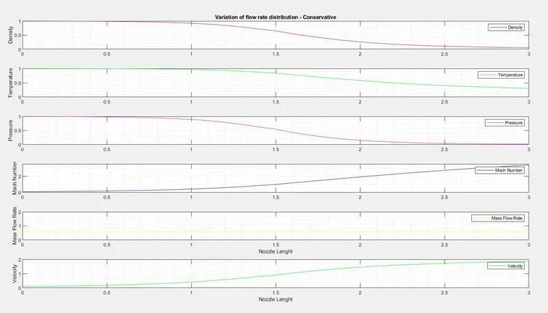
• Each plot is computed as subplots of four primitive variables such as Density, Temperature, Pressure, and Mach Number at the throat as well as the Convergent/Divergent section.

Conservative form function code:

function [mass_flow_rate_c, pressure_c, mach_number_c,  rho_c, v_c, t_c, rho_throat_c, v_throat_c, t_throat_c, mass_flow_rate_throat_c, pressure_throat_c, mach_number_throat_c] = Conservative_form(x, dx, n, gamma, nt, c)

%Determining Initial profile of Density and Temperature
for i = 1:n
    
    if (x(i) >= 0 && x(i) <= 0.5)
        rho_c(i) = 1;
        t_c(i) = 1;
    elseif (x(i) >= 0.5 && x(i) <= 1.5)
        rho_c(i) = 1 - 0.366*(x(i) - 0.5);
        t_c(i) = 1 - 0.167*(x(i) - 0.5);
    elseif (x(i) >= 1.5 && x(i) <= 3)
        rho_c(i) = 0.634 - 0.3879*(x(i) - 1.5);
        t_c(i) = 0.833 - 0.3507*(x(i) - 1.5);
    end
    
end

%Area & Throat profiles
a = 1 + 2.2*(x - 1.5).^2;
throat = find(a==1);

%Initial profile fot Velocity and Pressure
v_c = 0.59./(rho_c.*a);
pressure_c = rho_c.*t_c;

%Calculate the Initial Solution Vectors(U)
U1 = rho_c.*a;
U2 = rho_c.*a.*v_c;
U3 = rho_c.*a.*(t_c./(gamma - 1)) + ((gamma/2).*v_c.^2);


%Outer Time Loop
for k =1:nt
    
    %Time-step control
    dt = min(c.*dx./(sqrt(t_c) + v_c));
    
    %Saving a copy of Old Values
    U1_old = U1;
    U2_old = U2;
    U3_old = U3;

    %Calculating the Flux vector(F)
    F1 = U2;
    F2 = ((U2.^2)./U1) + ((gamma - 1)/gamma)*(U3 - (gamma/2)*((U2.^2)./U1));
    F3 = ((gamma*U2.*U3)./U1) - (gamma*(gamma - 1)*((U2.^3)./(2*U1.^2)));
    
    
    %Predictor Method
    for j = 2:n-1
    
        %Calculating the Source term(J)
        J2(j) = (1/gamma)*rho_c(j)*t_c(j)*((a(j + 1) - a(j))/dx);
        
        
        %Continuity Equation
        dU1_dt_P(j) = -((F1(j + 1) - F1(j))/dx);
        
        %Momentum Equation
        dU2_dt_P(j) = -((F2(j + 1) - F2(j))/dx) + J2(j);
        
        %Energy Equation
        dU3_dt_P(j) = -((F3(j + 1) - F3(j))/dx);
        
        
        %Updating New values
        U1(j) = U1(j) + dU1_dt_P(j)*dt;
        U2(j) = U2(j) + dU2_dt_P(j)*dt;
        U3(j) = U3(j) + dU3_dt_P(j)*dt;
        
    end
    
    %Updating Flux vectors
    F1 = U2;
    F2 = ((U2.^2)./U1) + ((gamma - 1)/gamma)*(U3 - ((gamma*0.5*(U2.^2))./(U1)));
    F3 = ((gamma*U2.*U3)./U1) - ((gamma*0.5*(gamma - 1)*(U2.^3))./(U1.^2));

    
    %Corrector Method
    for j = 2:n-1
        
        %Updating the Source term(J)
        J2(j) = (1/gamma)*rho_c(j)*t_c(j)*((a(j) - a(j - 1))/dx);

        %Simplifying the Equation's spatial terms
        dU1_dt_C(j) = -((F1(j) - F1(j - 1))/dx);
        dU2_dt_C(j) = -((F2(j) - F2(j - 1))/dx) + J2(j);
        dU3_dt_C(j) = -((F3(j) - F3(j - 1))/dx);

    end

    %Compute Average Time derivative
    dU1_dt = 0.5*(dU1_dt_P + dU1_dt_C);
    dU2_dt = 0.5*(dU2_dt_P + dU2_dt_C);
    dU3_dt = 0.5*(dU3_dt_P + dU3_dt_C);

    %Final Solution Update
    for i = 2:n-1
        U1(i) = U1_old(i) + dU1_dt(i)*dt;
        U2(i) = U2_old(i) + dU2_dt(i)*dt;
        U3(i) = U3_old(i) + dU3_dt(i)*dt;
        
    end
    
    
    %Applying Boundary Conditions
    %At Inlet
    U1(1) = rho_c(1)*a(1);
    U2(1) = 2*U2(2) - U2(3);
    
    v_c(1) = U2(1)./U1(1);
    U3(1) = U1(1)*((t_c(1)/(gamma - 1)) + ((gamma/2)*(v_c(1)).^2));
    
    %At Outlet
    U1(n) = 2*U1(n - 1) - U1(n - 2);
    U2(n) = 2*U2(n - 1) - U2(n - 2);
    U3(n) = 2*U3(n - 1) - U3(n - 2);
    
    %Final Updated value
    rho_c = U1./a;
    v_c = U2./U1;
    t_c = (gamma - 1)*((U3./U1 - (gamma/2)*(v_c).^2));
    
    %Defining Mass flow rate, Pressure and Mach number
    mass_flow_rate_c = rho_c.*a.*v_c;
    pressure_c = rho_c.*t_c;
    mach_number_c = (v_c./sqrt(t_c));
    
    %Calculating Variables at throat section
    rho_throat_c(k) = rho_c(throat);
    t_throat_c(k) = t_c(throat);
    v_throat_c(k) = v_c(throat);
    mass_flow_rate_throat_c(k) = mass_flow_rate_c(throat);
    pressure_throat_c(k) = pressure_c(throat);
    mach_number_throat_c(k) = mach_number_c(throat);

     %Comparison of non-dimensional Mass flow rates at different time steps
    figure(3)
    if k == 50
       plot(x, mass_flow_rate_c, 'm', 'linewidth', 1.25);
       hold on
    elseif k == 100
       plot(x, mass_flow_rate_c, 'c', 'linewidth', 1.25);
       hold on
    elseif k == 200
       plot(x, mass_flow_rate_c, 'g', 'linewidth', 1.25);
       hold on
    elseif k == 400
       plot(x, mass_flow_rate_c, 'y', 'linewidth', 1.25);
       hold on
    elseif k == 800
       plot(x, mass_flow_rate_c, 'k', 'linewidth', 1.25);
       hold on
    end
           
    
    %Labelling
    title('Mass flow rates at different Timesteps - CONSERVATIVE FORM')
    xlabel('Distance')
    ylabel('Mass flow rate')
    legend({'50^t^h Timestep','100^t^h Timestep','200^t^h Timestep','400^t^h Timestep','800^t^h Timestep'})
    axis([0 3 0.4 1])
    grid on
end

figure(4)
% Density plot
subplot(6,1,1)
plot(x,rho_c,'color','r')
ylabel('Density')
legend({'Density'})
title('Variation of flow rate distribution - Conservative')
axis([0 3 0 1])
grid minor;


% Temperature plot
subplot(6,1,2)
plot(x,t_c,'color','g')
ylabel('Temperature')
legend({'Temperature'})
axis([0 3 0 1])
grid minor;

%  Pressure plot
subplot(6,1,3)
plot(x,pressure_c,'color','m')
ylabel('Pressure')
legend({'Pressure'})
axis([0 3 0 1])
grid minor;

% Mach Number plot
subplot(6,1,4)
plot(x,mach_number_c,'color','b')
ylabel('Mach Number')
legend({'Mach Number'})
axis([0 3 0 3.5])
grid minor;

%  Mass Flow Rate plot
subplot(6,1,5)
plot(x,mass_flow_rate_c,'color','y')
xlabel('Nozzle Lenght')
ylabel('Mass Flow Rate')
legend({'Mass Flow Rate'})
axis([0 3 0 2])
grid minor;

%  Velocity plot
subplot(6,1,6)
plot(x,v_c,'color','g')
xlabel('Nozzle Lenght')
ylabel('Velocity')
legend({'Velocity'})
axis([0 3 0 2])
grid minor;


    
end

Background of Code:

• For this initial boundary conditions are established for Density, Temperature & Velocity, and profiles for calculating area & throat.
• To simplify and avoid errors, the equation is split into Solution Vector(U), Flux Vector(F), and Source Term(J).
• MacCormack technique is used to solve the numerical solution of governing equations such as Continuity, Momentum & Energy Equation.
• The technique implies two methods for solving namely the Predictor method followed by the Corrector method.
• The predictor & Corrector methods are assigned within the for loop individually for calculating values.
• The calculated values are averaged in the next step and updating the solution with old values.
• Boundary Conditions are applied within the for loop and subsequently used to calculate the Mass Flow Rate, Mach Number & Pressure, and calculate the values throat section.
• Finally plotting is done for Distance(x) & Mass Flow Rate for different Timesteps.
• Plotting is done for the following solutions
• Each plot is computed as subplots of four primitive variables such as Density, Temperature, Pressure, and Mach Number at the throat as well as the Convergent/Divergent section.

Results:

Non-Conservative form graphical representation:

Figure 1:

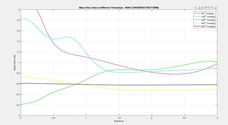
Figure 2:

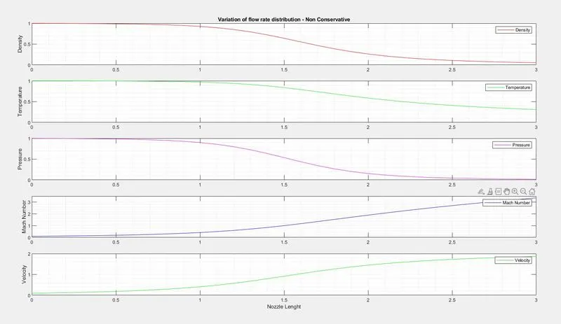
Figure 3:

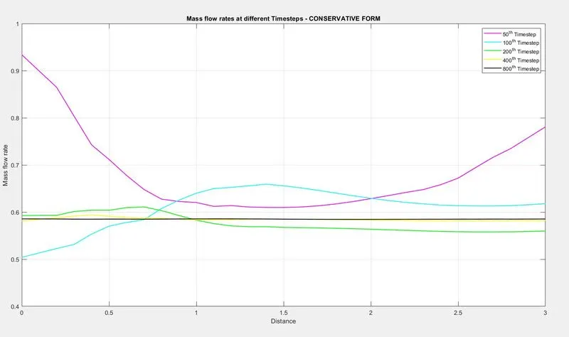
Figure 4:

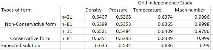
Grid Independence Study:

Conclusion:

• From figure(1) we can see that the non-conservative form take time to converge the solution also it has stable result only after 400-time steps.
• From figure(3) we can say that the conservative form will converge faster than the non-conservative form and also has a high accuracy of the result and also has stable results at 400-time steps.

After seeing all the above results we can say that the conservative form is converging faster than the non-conservative form.