Week 5.1 - Mid term project - Solving the steady and unsteady 2D heat conduction problem

AIM:

To solve steady-state and transient-state of 2D heat conduction problem using Implicit and Explicit by different iterative solvers.

Methodology:

Explicit Method;

This method requires stable criteria which leads to a stable solution. Due to stable criteria, small-time steps have taken to obtain stable solutions, decrease in time-steps the number of computations increases and the time required for the solution to converge is less and the accuracy is high.

Implicit Method:

This method is not stable as result, no stable criteria are required to obtain stable results. Due to no stable criteria, the time required for the solution to converge is high, and the solution's accuracy is less compared with the explicit method. As there is no stable criteria requirement large time steps can be used.

Iterative Solvers:

• Jacobi:

For this method, we assume that the initial nodes are used to find the other unknown nodes and this process continues until the solution is converged.

• Gauss-seidel method:

This method uses the values obtained from the Jacobi iteration for the next equation for competing for one iteration.

• Successive over-relaxation with Gauss-seidel method:

In this method we need to use relaxation factor to ease the process. `omega` is the relaxation factor.

When `omega` is between 0-1 it is called under relaxation.

When `omega` is between 1-2 it is called over relaxation.

2D Heat Conduction Equation:

`(delT)/(delt)+alpha((del^2T)/(delx^2)+(del^2T)/(dely^2))=0` ----------1

Steady state equation:

For steady state there is no change in temperature,

`(del^2T)/(delx^2)+(del^2T)/(dely^2)=0` -------2

Discretization of time derivative using FDS and can be solved my time marching,

`(del^2T)/(delx^2)=(T_L-2T_p+T_R)/(Deltax^2)` -------------3

`(del^2T)/(dely^2)=(T_T-2T_p+T_B)/(Deltay^2)` --------------4

`therefore` simplifying ,

where `k = 2((Delta x^2 +Delta y^2)/(Delta x^2*Delta y^2))`

`T_p=1/k((T_L+T_R)/(Deltax^2)+(T_T+T_B)/(Deltay^2))`----------5

For steady-state iterative solver equation:

• Jacobi method equation:`T^(n+1) = T^n*k + k1(T_L +T_R) +k2(T_BT+T_B)`

`(T_p)^(n+1) = ((T_L + T_R)^(n)+(T_T+T_B)^(n))/k`

• Gauss-seidel method equation:

`(T_p)^(n+1) = ((T_L + T_R)^(n+1)+(T_T+T_B)^(n+1))/k`

• Successive over-relaxation with Gauss-seidel method equation:

`(T_p)^(n+1) =(T_P)^n*(1-omega)+omega* (((T_L + T_R)^(n+1)+(T_T+T_B)^(n+1))/k)`

Transient state equation:

`(del T)/ (del t)= alpha nabla^2 T` ----------6

Discretization of time derivative using FDS and can be solved by second-order CDS,

`(del T)/ (del t)= (T^(n+1) -T^n)/(Delta t)` --------7

`T^(n+1) = T^n + alpha Delta t ((T_L -2T^n +T_R)/(Delta x^2) + (T_B -2T^n +T_T)/(Delta y^2))` ------8

where ,`k1 = alpha (Delta t)/(Delta x^2) , k2 = alpha (Delta t)/(Delta y^2)`

`K=(1+2*K_1+2*K_2)^-1`

`therefore` `T^(n+1) = T^n + k1(T_L -2T^n +T_R) +k2(T_B -2T^n +T_T)` ----------9

For transient-state iterative solver equation:

• Jacobi method equation:

`T^(n+1) = T^n*k + k1(T_L +T_R)^n +k2(T_T +T_B)^n`

• Gauss-seidel method equation:

`T^(n+1) = T^n*k + k1(T_L^(n+1) +T_R^n) +k2(T_T^n +T_B^(n+1))`

• Successive over-relaxation with Gauss-seidel method equation:

`T^(n+1) = T^n*k*(1-omega) +omega*(k1(T_L^(n+1) +T_R^n) +k2(T_T^n +T_B^(n+1)))`

MATLAB CODE:

Main code for calling all function code:

% code to solve 2nd order one dimensional PDE
% code for steady state analysis and transient state analysis
close all
clear all
clc
% number of grids in x and y direction
nx=10;
ny=10;
x=linspace(0,1,nx);
y=linspace(0,1,ny);
%grid spacing
dx=x(2)-x(1);
dy=y(2)-y(1);

%boundary condition
t=300*ones(nx,ny);
t(1,:) = 600; % Top boundary
t(end,:) = 900; % Bottom boundary
t(:,1) = 400; %Left boundary
t(:,end) = 800; %Right boundary

% k is the coefficient 
k = (2*(dx^2+dy^2)/(dx^2*dy^2));
told = t;
tpre = t;
tol = 1e-4;
% time loop condition
T = 5;
dt = 0.01;
nt = T/dt;
% Functions for steady state condition
%  Function for Jacobi method
[error_jacobi,iter_1] = jacobi(nx,ny,x,y,dx,dy,told,tol,k,t);
%  Function for Gauss-seidel method
[error_gs,iter_2] = gs(nx,ny,x,y,dx,dy,told,tol,k,t);
%  Function for  Successive over-relaxation on Gauss-seidel method
[error_SOR_gs,iter_3] = SOR_gs(nx,ny,x,y,dx,dy,told,tol,k,t);

% Functions for steady state condition
%  Function for Jacobi method
[error_jacobi_transient,iter_4] = jacobi_transient_state(nx,ny,x,y,dx,dy,told,tpre,tol,t,T,nt,dt)
%  Function for Gauss-seidel method
[error_gs_transient,iter_5] = gs_transient_state(nx,ny,x,y,dx,dy,told,tpre,tol,t,T,nt,dt)
%  Function for  Successive over-relaxation on Gauss-seidel method
[error_SOR_gs_transient,iter_6] =  SOR_gs_transient_state(nx,ny,x,y,dx,dy,told,tpre,tol,t,T,nt,dt,k)

Steady State condition Matlab code:

Function for Jacobi method:

function [error_jacobi,iter_1] = jacobi(nx,ny,x,y,dx,dy,told,tol,k,t)
iter_1=1;
error_jacobi = 9e9;
iterative_solver=1;
if iterative_solver==1
    while(error_jacobi>tol)
    for i=2:nx-1
        for j=2:ny-1
            TL = told(i-1,j);
            TR = told(i+1,j);
            TT = told(i,j+1);
            TB = told(i,j-1);
            H = (TL+TR)/dx^2;
            V = (TB+TT)/dy^2;
            t(i,j) = (H+V)/k;
        end
     error_jacobi=max(max(abs(told-t)));
     told=t;
     iter_1=iter_1+1;
    end
    end
end
%plotting graph
figure(1)
     [x,y]= contourf(t)
     set(gca,'YDIR','reverse')
        colormap(jet)
        colorbar
        clabel(x,y)
        pause(0.03)
        title_text1 = sprintf('Iteration = %d', iter_1);
        title_text2 = sprintf('Jacobi Method')
        title({title_text1; title_text2})            

Function for Gauss-seidel method:

function [error_gs,iter_2] = gs(nx,ny,x,y,dx,dy,told,tol,k,t)
iter_2=1;
error_gs = 9e9;
iterative_solver=2;
if iterative_solver==2
    while(error_gs>tol)
    for i=2:nx-1
        for j=2:ny-1
            TL = t(i-1,j);
            TR = told(i+1,j);
            TT = told(i,j+1);
            TB = t(i,j-1);
            H = (TL+TR)/dx^2;
            V = (TB+TT)/dy^2;
            t(i,j) = (H+V)/k;
        end
     error_gs=max(max(abs(told-t)));
     told=t;
     iter_2=iter_2+1;
     
     %plotting graph
     
    end
    end
end
figure(2)
     [x,y]= contourf(t);
     set(gca,'YDIR','reverse')
        colormap(jet)
        colorbar
        clabel(x,y)
        pause(0.03)
        title_text1 = sprintf('Iteration = %d', iter_2);
        title_text2 = sprintf('Gauss-seidel Method')     
        title({title_text1; title_text2})
            

Function for Successive over-relaxation with Gauss-seidel method:

function [error_SOR_gs,iter_3] = SOR_gs(nx,ny,x,y,dx,dy,told,tol,k,t)
omega = 1.1;
iter_3=1;
error_SOR_gs = 9e9;
iterative_solver=3;
if iterative_solver==3
    while(error_SOR_gs>tol)
    for i=2:nx-1
        for j=2:ny-1
            TL = t(i-1,j);
            TR = told(i+1,j);
            TT = told(i,j+1);
            TB = t(i,j-1);
            H = (TL+TR)/dx^2;
            V = (TB+TT)/dy^2;
            t_gs(i,j) = (H+V)/k;
            t(i,j)=(1-omega)*(told(i,j))+omega*t_gs(i,j);
            
        end
     error_SOR_gs=max(max(abs(told-t)));
     told=t;
     iter_3=iter_3+1;
    end
    end
end
%plotting graph
figure(3)
     [x,y]= contourf(t);
        set(gca,'YDIR','reverse')
        colormap(jet)
        colorbar
        clabel(x,y)
        pause(0.03)
        title_text1 = sprintf('Iteration = %d', iter_3);
        title_text2 = sprintf('SOR method with Gauss-seidel Method')     
        title({title_text1; title_text2})
        
     
            

Results for the steady-state condition:

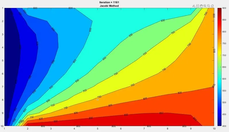
Jacobi Method:

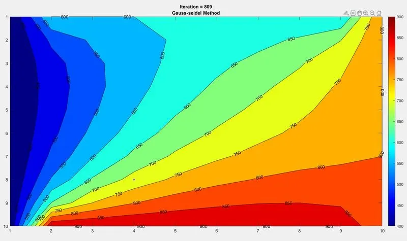
Gauss-seidel method:

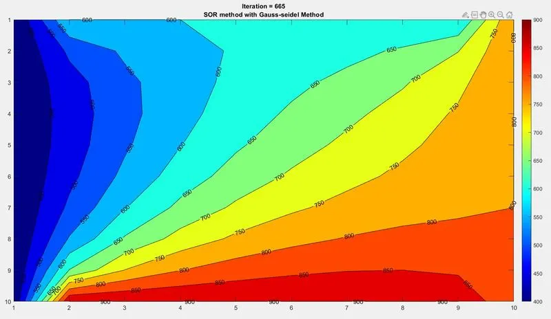
Successive over-relaxation with Gauss-seidel method:

Function code for Transient state conditions:

Function for Jacobi Method:

function [error_jacobi_transient,iter_4] = jacobi_transient_state(nx,ny,x,y,dx,dy,told,tpre,tol,t,T,nt,dt)
iter_4=1;

alpha = 0.4;
k1 = alpha*dt/dx^2;
k2 = alpha*dt/dy^2;
k =(1+(2*k1)+(2*k2))^-1;
iterative_solver=1;
if iterative_solver==1
    for m = 1:nt
        error_jacobi_transient = 9e9;
    while(error_jacobi_transient>tol)
    for i=2:nx-1
        for j=2:ny-1
            TL = told(i-1,j);
            TR = told(i+1,j);
            TT = told(i,j+1);
            TB = told(i,j-1);
            H = (TL+TR);
            V = (TB+TT);
            t(i,j) = (tpre(i,j)*k)+(k*k1*H)+(k*k2*V);
        end
         end
     error_jacobi_transient=max(max(abs(t-told)));
     told=t;
     iter_4=iter_4+1;
    end
    tpre=t;
    end
end
%plotting graph
figure(4)
     [x,y]= contourf(t)
     set(gca,'YDIR','reverse')
        colormap(jet)
        colorbar
        clabel(x,y)
        pause(0.03)
        title_text1 = sprintf('Iteration = %d', iter_4);
        title_text2 = sprintf('Jacobi Method in Transient state')
        title({title_text1; title_text2})            

Function for Gauss-seidel method:

function [error_gs_transient,iter_5] = gs_transient_state(nx,ny,x,y,dx,dy,told,tpre,tol,t,T,nt,dt)
iter_5=1;
alpha = 0.4;
k1 = alpha*dt/dx^2;
k2 = alpha*dt/dy^2;
k =(1+(2*k1)+(2*k2))^-1;
iterative_solver=5;
if iterative_solver==5
    for m = 1:nt
        error_gs_transient = 9e9;
    while(error_gs_transient>tol)
    for i=2:nx-1
        for j=2:ny-1
            TL = t(i-1,j);
            TR = told(i+1,j);
            TT = told(i,j+1);
            TB = t(i,j-1);
            H = (TL+TR);
            V = (TB+TT);
            t(i,j) = (tpre(i,j)*k)+(k*k1*H)+(k*k2*V);
        end
     error_gs_transient=max(max(abs(told-t)));
     told=t;
     iter_5=iter_5+1;
    end
    end
    tpre=t;
    end
end
%plotting graph
figure(5)
     [x,y]= contourf(t)
     set(gca,'YDIR','reverse')
        colormap(jet)
        colorbar
        clabel(x,y)
        pause(0.03)
        title_text1 = sprintf('Iteration = %d', iter_5);
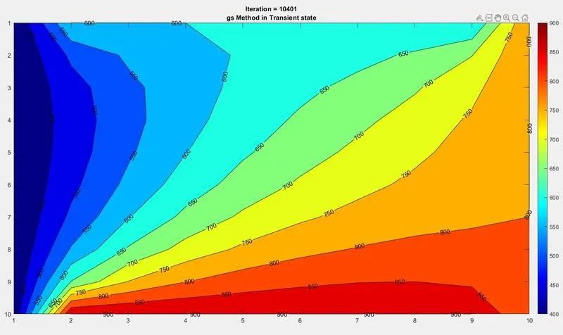
        title_text2 = sprintf('gs Method in Transient state')
        title({title_text1; title_text2})            

Function for successive over-relaxation with Gauss-seidel method:

function [error_SOR_gs_transient,iter_6] = SOR_gs_transient_state(nx,ny,x,y,dx,dy,told,tpre,tol,t,T,nt,dt,k)
omega = 1.1;
iter_6=1;
iterative_solver=3;
if iterative_solver==3
    for m = 1:nt
        error_SOR_gs_transient = 9e9;
    while(error_SOR_gs_transient>tol)
    for i=2:nx-1
        for j=2:ny-1
            TL = t(i-1,j);
            TR = told(i+1,j);
            TT = told(i,j+1);
            TB = t(i,j-1);
            H = (TL+TR)/dx^2;
            V = (TB+TT)/dy^2;
            t_gs(i,j) = (H+V)/k;
            t(i,j)=(1-omega)*(told(i,j))+omega*t_gs(i,j);
            
        end
     error_SOR_gs_transient=max(max(abs(told-t)));
     told=t;
     iter_6=iter_6+1;
    end
    end
    end
end

%plotting graph
figure(6)
     [x,y]= contourf(t);
        set(gca,'YDIR','reverse')
        colormap(jet)
        colorbar
        clabel(x,y)
        pause(0.03)
        title_text1 = sprintf('Iteration = %d', iter_6);
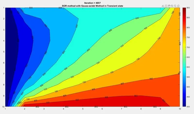
        title_text2 = sprintf('SOR method with Gauss-seidel Method in Transient state')     
        title({title_text1; title_text2})
        
     
            

Results for transient state condition:

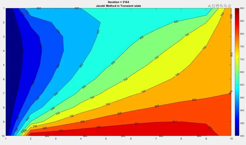
Jacobi Method:

Gauss-seidel method:

successive over-relaxation with Gauss-seidel method:

Conclusion:

Tables for iterations Vs solvers:

Steady-state condition:

Iterative Solver	Number of iterations
Jacobi Method	1161
Gauss-seidel method	809
successive over-relaxation	665

Transient-state condition:

Iterative Solver	Number of iterations
Jacobi Method	2164
Gauss-seidel method	10401
successive over-relaxation	4657

Hence for time step size, the explicit scheme has a faster converging rate and less number of iterations and for the implicit scheme a large number of iteration to converge the solution.