Week 9 - Mini project - Flow over an Airfoil
AIM:
- To simulate flow over an airfoil for different angles of attack.
- To find out the lift and drag coefficients using pressure force.
THEORY:
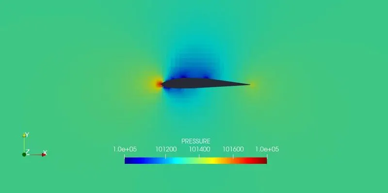
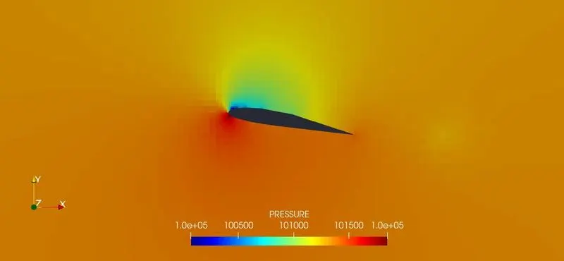
Any object that needs to be in fly should have the pressure difference at the upper body and lower body. NACA 2412 is an unsymmetrical airfoil so there will be pressure differences at the upper body and lower body. Unsymmetrical airfoils will have a lift at a 0-degree angle because the chamber at the upper surface and lower surface are different. If a wing needs to generate lift then it should have high pressure at a lower surface and high low pressure at the upper surface, high pressure at the lower generate lift. Flow separation at the airfoil will also generate lift. Flow separated at the tip of the airfoil should join the smoothly the root of the airfoil. For 0 AOA the flow separation will be smooth while increasing the AOA the separation will be rough due to the high-pressure difference at both upper and lower surfaces.
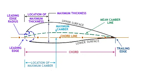
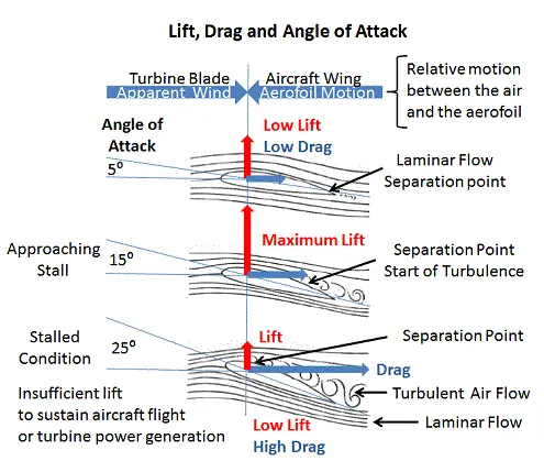
The above images describe the flow separation when the AOA changes.
PROCEDURE FOR SETTING UP THE SIMULATION CASE:
Importing Geometry & Diagnosis:
- I have used Solidworks to design the airfoil and domain and converted it into an STL file.
- Import the geometry in the STL file which is in the form of triangles.
- After importing run the diagnosis for checking the geometry for any problem in cad.
- Most important this that we need to check the normal also, the normal should be pointing towards the domain.
Case set-up :
- The application type is Timebase.
- A predefined air mixture is used.
- Using turbulent Prandtl number 0.9.
- Using turbulent Schmidt number 0.78.
- O2 and N2 are species of air.
Simulation Parameters:
- A transient-state solver is used.
- Starting time is 0s and the ending time is 0.003.
- The minimum time step is 1e-9s.
- The maximum time step is 1s.
Boundary Condition and Region Initialization:
- The Inlet, Outlet, Front 2D, Back 2D, Top and bottom wall, and wing total of six boundaries are used.
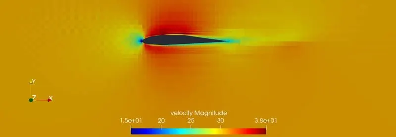
- Inlet and velocity inlet and velocity as 30.5 m/s and species as air.
- Outlet as pressure outlet of 101325 pa and backflow species as air.
- Front and back 2D is considered as 2D.
- The top and wall bottom wall is considered symmetry.
- The wing is considered a wall and the law of wall condition are provided.
Physical Model:
- We are using RANS_K_EPS_RNG ( Re-Normalisation Group) turbulence model.
Grid Control:
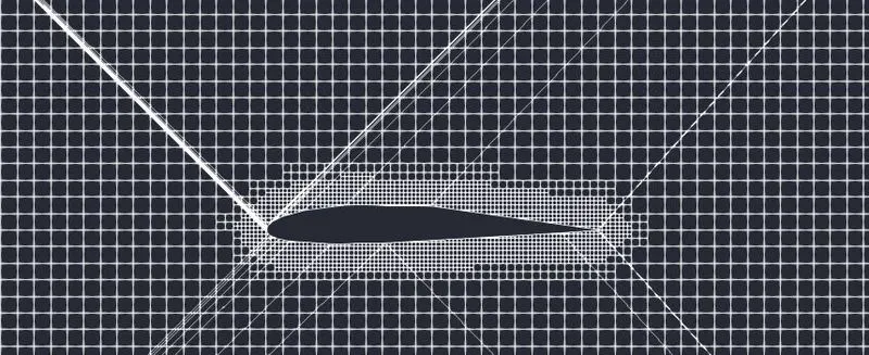
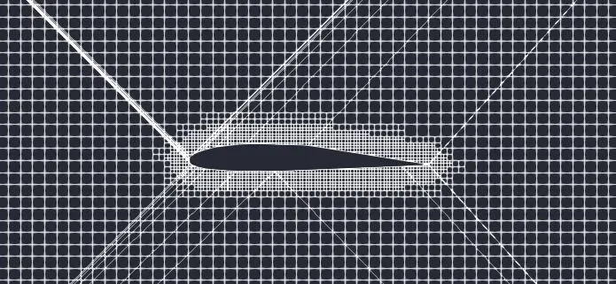
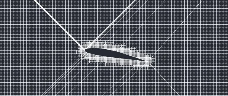
- In grid control, we will be defining the mesh size for the domain (0.002 m is the mesh size).
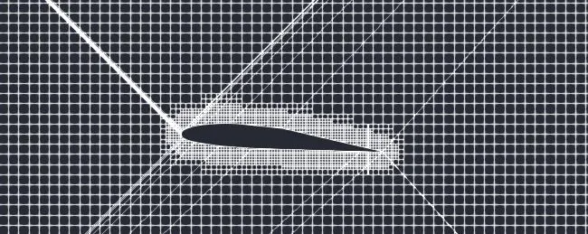
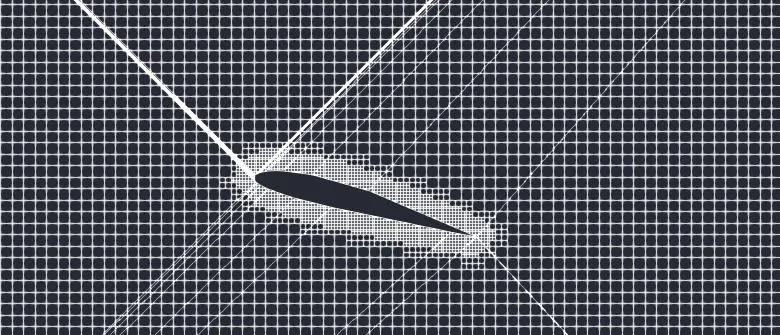
- Here we are using fixed embedding to refine the mesh at airfoil to capture the flow physics.
Output and Post-processing:
- In the post-variable selection, we can select the output that we need for post-processing.
- In output files, we can set time intervals for writing the 3D output.
- We can also set time intervals for writing, restarting files.
Running Simulation:
- After finishing setting up the simulation case we need to export the input files in a folder.
- Now open the Cygwin terminal and navigate to the folder where you exported the input files.
- Now run the executable mpiexec.exe -n 2 converge.exe restricted.
- After finishing the simulation we need to convert the output file to paraview format.
- mpiexec.exe -n 2 post_convert_30_msmpi_64.exe command is used to convert the file as ParaView format.
RESULTS:
CASE 1: AOA 0
MESH GENERATION:
VELOCITY CONTOUR:
PRESSURE CONTOUR:
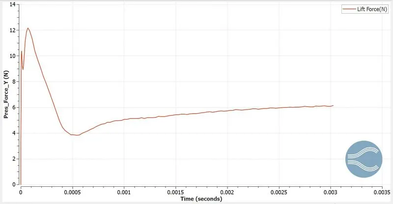
LIFT FORCE PLOT:
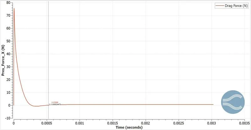
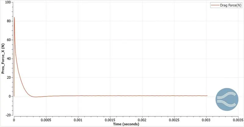
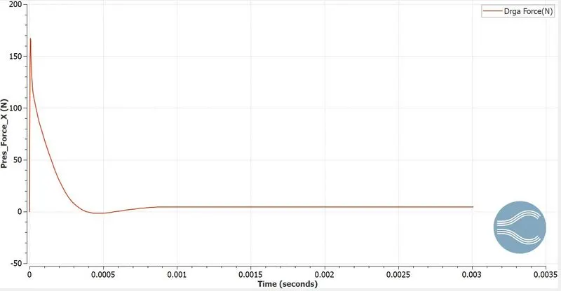
DRAG FORCE PLOT:
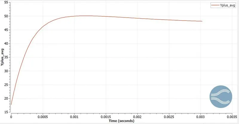
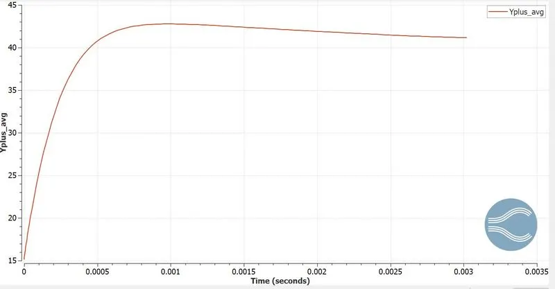
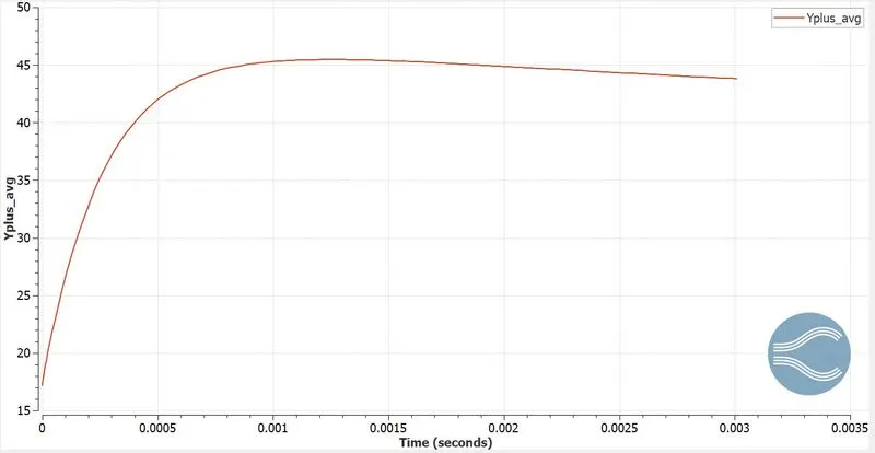
AVERAGE Y PLUS PLOT:
CASE 2: AOA 1
MESH GENERATION:
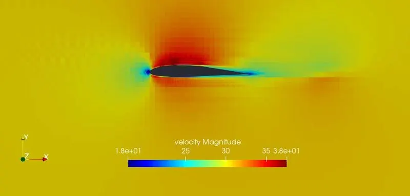
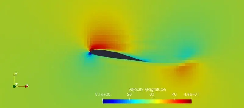
VELOCITY CONTOUR:
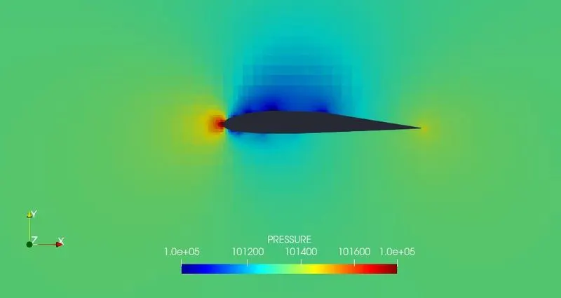
PRESSURE CONTOUR:
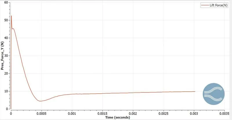
LIFT FORCE PLOT:
DRAG FORCE PLOT:
AVERAGE YPLUS PLOT:
CASE 3: AOA 5
MESH GENERATION:
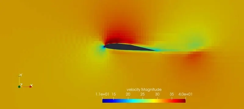
VELOCITY CONTOUR:
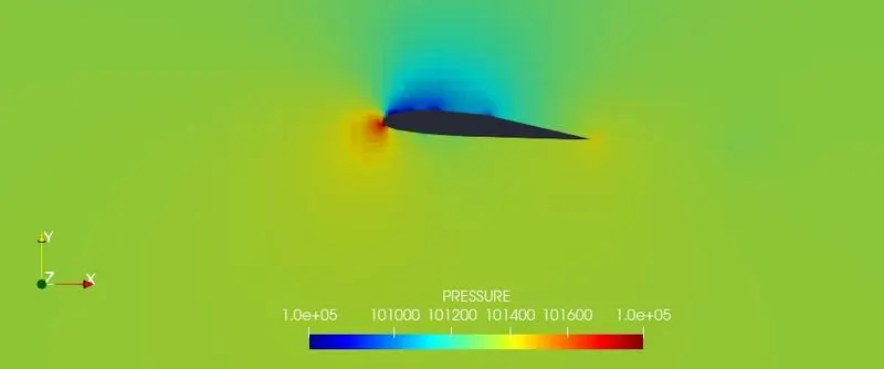
PRESSURE CONTOUR:
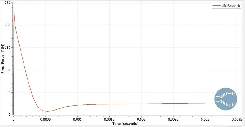
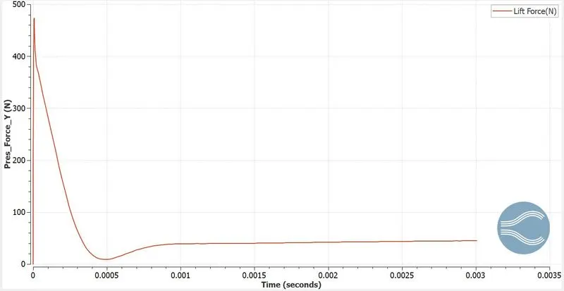
LIFT FORCE PLOT:
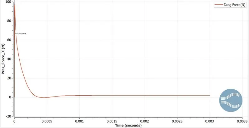
DRAG FORCE PLOT:
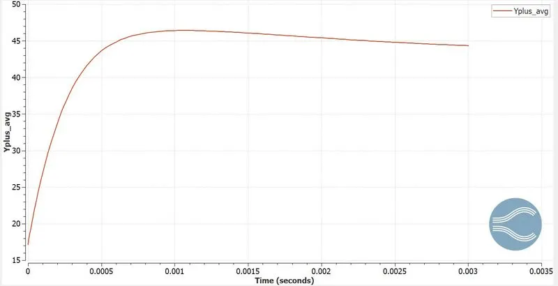
AVERAGE YPLUS PLOT:
CASE 4: AOA 10
MESH GENERATION:
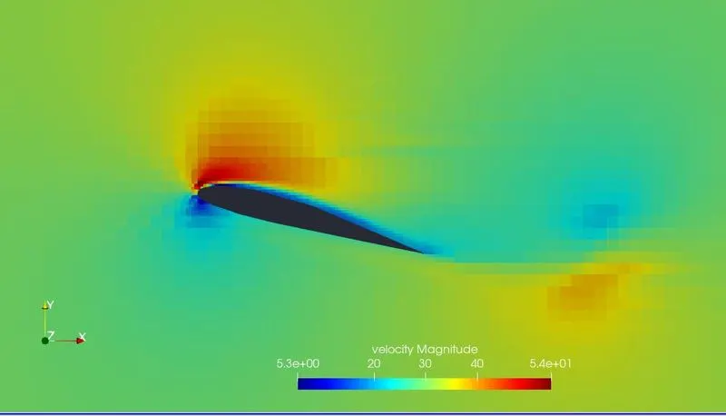
VELOCITY CONTOUR:
PRESSURE CONTOUR:
LIFT FORCE PLOT:
DRAG FORCE PLOT:
AVERAGE YPLUS PLOT:
CASE 5: AOA 15
MESH GENERATION:
VELOCITY CONTOUR:
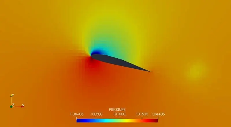
PRESSURE CONTOUR:
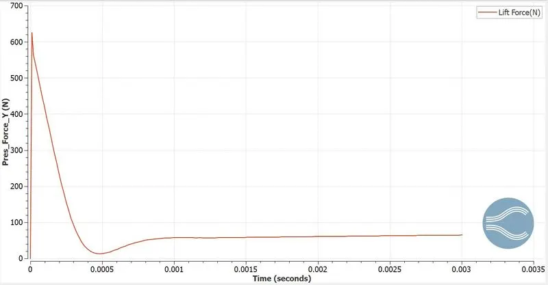
LIFT FORCE PLOT:
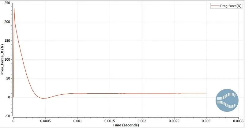
DRAG FORCE PLOT:
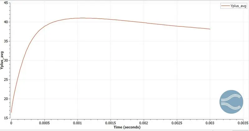
AVERAGE YPLUS PLOT:
CALCULATION OF COEFFICIENT OF LIFT AND DRAG:
0 AOA:
Lift (n): 6.13488
Drag (n): 0.689475
The formula to find the coefficient of lift is;
`Cl=L/(1/2*rho*v^2*s)`
The formula to find the coefficient of drag is;
`Cd=D/(1/2*rho*v^2*s)`
`rho` denotes the density of air which is 1.225
`v^2` denotes the velocity of air at the inlet is 30.5 m/s
`s` denotes the surface area of the airfoil which is 0.1m.
`Cl = 6.13488/(1/2*1.225*30.5^2*0.1)`
`Cl = 0.107`
`Cd = 0.689475/(1/2*1.225*30.5^2*0.1)`
`Cd = 0.0121`
Using this method we can find cl and cd values for different AOA.
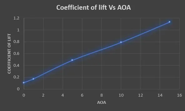
Coefficient of Lift Vs AOA graph:
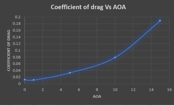
Coefficient of Drag Vs AOA graph:
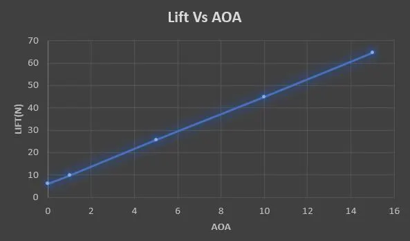
Lift Vs AOA graph:
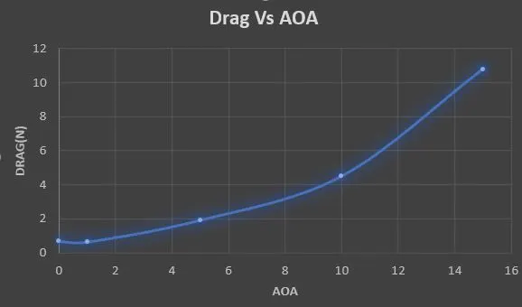
Drag Vs AOA graph:
CONCLUSION:
- We see that the AOA changed the lift and drag values are increasing due to pressure difference.
- From this simulation, we understand the concept of flow over an airfoil and how to calculate the coefficient of lift and coefficient of drag from pressure force.