Week 3.5 - Deriving 4th order approximation of a 2nd order derivative using Taylor Table method

AIM:

To derive 4th order approximation using Taylor's table by Central difference, Skewed right-sided difference & Skewed left-sided difference.

Central Difference method:

`(del^2u)/(dx^2)=(a*f(i-2)+b*f(i-1)+c*f(i)+d*f(f+1)+e*f(i+2))/(dx^2)` -----------1

Talyor's Table for central difference method:

	`f(x)`	`f'(x).(Deltax)/(1!)`	`f''(x).(Deltax^2)/(!)`	`f'''(x).(Deltax^3)/(3!)`	`f'''''(x).(Deltax^4)/(4!)`
`a*f(i-2)`	a	-2a	4a/2	-8a/6	16a/24
`b*f(i-1)`	b	-b	b/2	-b/6	b/24
`c*f(i)`	c	0	0	0	0
`d*f(i+1)`	d	d	d/2	d/6	d/24
`e*f(i+2)`	e	2e	4e/2	8e/6	16e/24
`sum`	0	0	1	0	0

After obtaining the linear equation from Taylor's table we solve using the matrix inverse method.

`A*X=B` by using the matrix inverse method we can find out the values for coefficients.

`[[1,1,1,1,1],[-2,-1,0,1,2],[2,1/2,0,1/2,2],[-4/3,-1/6,0,1/6,4/3],[2/3,1/24,0,1/24,2/3]].[[a],[b],[c],[d],[e]] = [[0],[0],[1],[0],[0]]`

Skewed-Right Difference method:

`(del^2u)/(dx^2)=(a*f(i)+b*f(i+1)+c*f(i+2)+d*f(f+3)+e*f(i+4))/(dx^2)` ----------2

Talyor's Table for skewed-right difference method:

	f(x)	`f'(x)*(Deltax)/(1!)`	`f''(x)*(Deltax^2)/(2!)`	`f'''(x)*(Deltax*3)/(3!)`	`f''''(x)*(Deltax*4)/(4!)`
`a*f(i)`	a	0	0	0	0
`b*f(i+1)`	b	b	b/2	b/6	b/24
`c*f(i+2)`	c	2c	4c/2	8c/6	18c/24
`d*f(i+3)`	d	3d	3d/2	27d/6	82d/24
`e*f(i+4)`	e	4e	16e/2	64e/6	256e/21
`sum`	0	0	1	0	0

After obtaining the linear equation from Taylor's table we solve using the matrix inverse method.

`C*Y=D` by using the matrix inverse method we can find out the values for coefficients.

`[[1, 0 ,0, 0, 0],[1,1,1/2,1/6,1/24],[1,3,3/2,27/6,82/24],[1,4,16/2,64/6,256/24]]*[[a],[b],[c],[d],[e]]=[[0],[0],[1],[0],[0]]`

Skewed-left Difference method:

`(del^2u)/(dx^2)=(a*f(i-4)+b*f(i-3)+c*f(i-2)+d*f(f-1)+e*f(i))/(dx^2)` --------3

Talyor's Table for skewed-right difference method:

	`f(x)`	`f'(x).(Deltax)/(1!)`	`f'''(x).(Deltax^2)/(2!)`	`f'''(x).(Deltax^3)/(3!)`	`f''''(x).(Deltax^4)/(4!)`
`a*f(i-4)`	a	-4	16/2	-64/6	256/24
`b*f(i-3)`	b	-3	9/2	-27/6	81/24
`c*f(i-2)`	c	-2	4/2	-8/6	16/24
`d*f(i-1)`	d	-1	1/2	-1/6	1/24
`e*f(i)`	e	0	0	0	0
`sum`	0	0	1	0	0

After obtaining the linear equation from Taylor's table we solve using the matrix inverse method.

`E*Z=F` by using the matrix inverse method we can find out the values for coefficients.

MATLAB CODE:

Central difference function code:

function error = central_difference(exact_derivative,x,dx,X)
% Central differencing = (a*f(x-2*dx)+b*f(x-dx)+c*f(x)+d*f(x+dx)+e*f(x+2*dx))/(dx^2)
f1 = exp(x-2*dx)*cos(x-2*dx);
f2 = exp(x-dx)*cos(x-dx);
f3 = exp(x)*cos(x);
f4 = exp(x+dx)*cos(x+dx);
f5 = exp(x+2*dx)*cos(x+2*dx);
central_method = ((X(1)*f1)+(X(2)*f2)+(X(3)*f3)+(X(4)*f4)+(X(5)*f5))/(dx^2);
error = abs(central_method-exact_derivative);
end

Skewed-right difference function code:

function error = skewed_right_difference(exact_derivative,x,dx,Y)
%  skewed_right_difference = (a*f(x)+b*f(x+dx)+c*f(x+2*dx)+d*f(x+3*dx)+e*f(x+4*dx))/(dx^2)
f1 = exp(x)*cos(x);
f2 = exp(x+dx)*cos(x+dx);
f3 = exp(x+2*dx)*cos(x+2*dx);
f4 = exp(x+3*dx)*cos(x+3*dx);
f5 = exp(x+4*dx)*cos(x+4*dx);
skewed_right_method = ((Y(1)*f1)+(Y(2)*f2)+(Y(3)*f3)+(Y(4)*f4)+(Y(5)*f5))/(dx^2);
error = abs(skewed_right_method-exact_derivative);
end

Skewed-left difference function code:

function error = skewed_left_difference(exact_derivative,x,dx,Z)
%  skewed_left_difference = (a*f(x-4*dx)+b*f(x-3*dx)+c*f(x-2*dx)+d*f(x-dx)+e*f(x))/(dx^2)
f1 = exp(x-4*dx)*cos(x-4*dx);
f2 = exp(x-3*dx)*cos(x-3*dx);
f3 = exp(x-2*dx)*cos(x-2*dx);
f4 = exp(x-dx)*cos(x-dx);
f5 = exp(x)*cos(x);
skewed_left_method = ((Z(1)*f1)+(Z(2)*f2)+(Z(3)*f3)+(Z(4)*f4)+(Z(5)*f5))/(dx^2);
error = abs(skewed_left_method-exact_derivative);
end

Main code:

clear all
close all
clc

% finding the coefficients 
% finding the coefficientts of central difference method

A = [1 1 1 1 1; -2 -1 0 1 2; 4/2 1/2 0 1/2 4/2; -8/6 -1/6 0 1/6 8/6; 16/24 1/24 0 1/24 16/24];
B = [0;0;1;0;0];
a= inv(A);
X= a*B 

% finding the coefficientts of skewed right difference method

C = [1 1 1 1 1; 0 1 2 3 4; 0 1/2 4/2 9/2 16/2; 0 1/6 8/6 27/6 64/6; 0 1/24 16/24 81/24 256/24];
D = [0;0;1;0;0];
b = inv(C);
Y = b*D

% finding the coefficientts of skewed left difference method
E = [1 1 1 1 1; -4 -3 -2 -1 0; 16/2 9/2 4/2 1/2 0; -64/6 -27/6 -8/6 -1/6 0; 256/24 81/24 16/24 1/24 0];
F = [0;0;1;0;0];
c =  inv(E);
Z =  c*F

x=pi/3;
f = exp(x)*cos(x);
dx=linspace(pi/20,pi/400,20);
% analytical function = exp(x)*cos(x)
exact_derivative = -2*exp(x)*sin(x)

for i=1:length(dx)
    central_error(i) = central_difference(exact_derivative,x,dx(i),X)
    skewed_right_error(i) = skewed_right_difference(exact_derivative,x,dx(i),Y)
    skewed_left_error(i) = skewed_left_difference(exact_derivative,x,dx(i),Z)
end

%Plotting the solution as graph
loglog(dx,central_error,'color','b','linewidth',2)
hold on;
loglog(dx,skewed_right_error,'color','r','linewidth',2)
loglog(dx,skewed_left_error,'color','g','linewidth',2)
legend('Central difference','Skewed right-sided difference','Skewed left-sided difference')
xlabel('dx')
ylabel('error')
title('Error comparison using Taylors table')

RESULTS:

Values for coefficients X, Y & Z:

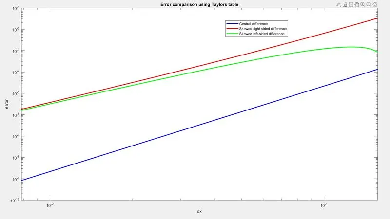
Loglog graph:

Conclusion:

• From the above graph, we came to know that the central difference method has low error compared with other methods.
• The central difference method uses the point of information from both sides, so it has a low error.

why a skewed scheme is useful?

A model which doesn't have enough point of information at both side then we cannot use central difference scheme, we need to skewed scheme.

What can a skewed scheme do that a CD scheme cannot?

At boundary nodes, we cannot use the CD scheme because there will be fewer nodes on the left and right sides at the same time, So at time we need to use a skewed scheme.