Project 2 - Rankine cycle Simulator

• First of all close all graph and clear all workspace memory.

  close all
  clear all
  clc​

• Now need to take input from user to calculate data.
• input :- This function is used to get input from user and store in variable. So, here we get three input from uer like Turbine Inlet pressure and Temprature and Turbine Outlet pressure.

  p1 = input('Enter Turbine inlet pressure (bar) =');
  t1 = input('Enter Turbine inlet Temprature (K) = ');
  p2 = input('Enter Condenser Pressure (bar) =');​

• Defining values for Point 1:-
• Call value using XStream function and write entropy and enthalpy at point 1 with input of temprature and pressure.

  % Point 1
  
  s1 = XSteam('s_pT',p1,t1);
  h1 = XSteam('h_pT',p1,t1);​

• Point 1 - 2 :- It is a isentropic expansion process in Turbine. So, entropy of point1 and point2 is same.
• While steam come out from turbine it is saturated. But it still has some fraction of vapour in it. So, we need to find entropy of liquid and vapour at p2 pressure and find fraction. Using this fraction and enthalpy of liquide and vapour water finding enthalpy of point2.

  % Point 2
  
  s2 = s1;
  t2 = XSteam('TSat_p',p2);
  sl2 = XSteam('sL_p',p2);
  sv2 = XSteam('sV_p',p2);
  x2 =  ((s2 - sl2) / (sv2 - sl2));
  hv2 = XSteam('hV_p',p2);
  hl2 = XSteam('hL_p',p2);
  h2 = hv2*x2 + (1-x2)*hl2;​

• Point 2 - 3 :- Now this mixture enters in condenser and loss heat. It is constant pressure heat rejection process. Temprature is ssame at both 2 and 3 point andat point 3, mixture becomes liquid. So, find entropy using liquid function. After that het enthalpy using entropy and pressure. Every paramter define of point 3.

  % Point 3
  
  p3 = p2;
  t3 = t2;
  s3 = XSteam('sL_p',p3);
  h3 = XSteam('h_ps',p3,s3);​

• Point 3 - 4 :- Now liquid enters in pump and compressed isentropically. So, entropy of point 3 and 4 is same.
• Point 4 - 1 :- In this last process water is heated at constant pressure. So, pressure of point 1 and 4 is same.
• After getting entropy and pressure find enthalpy using pressure and entropy function.
• To calculate temprature at point 4, we need gamma. For that Cp and Cv need to count of liquid water. So, using function get Cp,Cv then get gamma and t4.

  % Point 4
  
  p4 = p1;
  s4 = s3;
  h4 = XSteam('h_ps',p4,s4);
  cp4 = XSteam('CpL_p',p3);
  cv4 = XSteam('CvL_p',p3);
  gamma = cp4/cv4;
  t4 = (t3*((p3/p4)^((1-gamma)/gamma)));​

• Turbine work output is enthalpy difference of point 1 and 2.
• Pump input work is enthalpy difference of point 3 and 4.
• Heat input done in boiner is measured by enthalpy difference of point 1 and 4.
• Heat rejected in condenser is measured by enthalpy difference of point 2 and 3.
• Find net work output by substituting Turbine work and Pump work.
• Efficiency is getting by deviding net work with heat input.

  % Work output from 1 to 2
  
  W_T = h1 - h2;
  
  % Work input from 3 to 4
  
  W_P = h4 - h3;
  
  % Heat input in Boiler
  
  Q_In = h1 - h4;
  
  % Heat rejected in condenser
  
  Q_Rej = h2 - h3;
  
  % Efficiency
  
  W_net = W_T-W_P;
  n = W_net/Q_In;
  Efficiency = n*100;​

• To find saturation curve, we need value of entropy at different temprature of liquid and vapour water.
• linspace :- This command is used to make temprature array.
• With this array and use of for loop, we find value of entropy at differrent temprature.

  % Saturation curve liquid and vapour
  
  t = linspace(0,600,600);
  for i = 1:length(t)
      sl(i) = XSteam('sL_T',t(i));
      sv(i) = XSteam('sV_T',t(i));
  end​

• Now, we get all the required values and Outputs. So, plot the graphs,
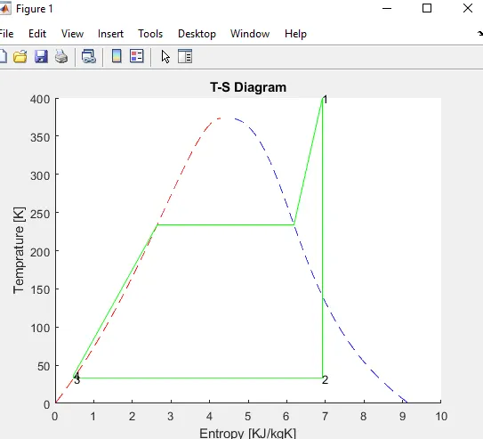
• First graph is of T-S Diagram.
• figure(i) :- This command is used to open different figure at a time with value of i.
• hold on :- THis command used to plot every graph in single graph.
• Plot saturation curve and all three processes from 1 to 2, 2 to 3, 3 to 4 using plot command.
• Process 4-1 is divided into threee portion.
• In first portion liquid water becomes saturated water. So, find saturated water temprature txl and entropy at that temprature sxl. Plot 4 to xl point.
• Then water becomes vapour. So, temprature of vapour is same as saturated water so txv = txl. From this find entropy of water vapour. Plot xl to xv.
• In last plot point xv to 4 which is Turbine inlet situation.
• Give label and title to graph.
• text :- This command used to give text to graph. Like we use here to number the point.
• Then use hold off command to stop writing plot in one figure.

  figure(1);
  hold on
  plot(sl,t,'--','Color','r')
  plot(sv,t,'--','Color','b')
  plot([s1,s2],[t1,t2],'color','g')
  plot([s2,s3],[t2,t3],'color','g')
  plot([s3,s4],[t3,t4],'color','g')
  
  % Divide cureve of Boiler input in 3 line
  
  txl = XSteam('TSat_p',p4);
  sxl = XSteam('sL_T',txl);
  txv = txl;
  sxv = XSteam('sV_T',txv);
  
  plot([s4,sxl],[t4,txl],'color','g')
  plot([sxl,sxv],[txl,txv],'color','g')
  plot([sxv,s1],[txv,t1],'color','g')
  title('T-S Diagram')
  xlabel('Entropy [KJ/kgK]')
  ylabel('Temprature [K]')
  
  text(s1,t1,'1');
  text(s2,t2,'2');
  text(s3,t3,'3');
  text(s4,t4,'4');
  hold off
  ​

• Second graph of H-S.
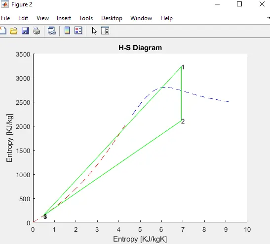
• figure(2) command to open secong graph.
• Hold on command to plot graph in single.
• First of all plot saturation curve for enthalpy for liquid and vapour as did upper portion.
• Then plot all for four process and give title, label and text. Then Hold off.

  % Saturation curve liquid and vapour
  
  t = linspace(0,600,600);
  for i = 1:length(t)
      hl(i) = XSteam('hL_T',t(i));
      hv(i) = XSteam('hV_T',t(i));
  end
  
  hold on
  plot(sl,hl,'--','Color','r')
  plot(sv,hv,'--','Color','b')
  plot([s1 s2],[h1,h2],'color','g')
  plot([s2 s3],[h2,h3],'color','g')
  plot([s3 s4],[h3,h4],'color','g')
  plot([s4 s1],[h4,h1],'color','g')
  title('H-S Diagram');
  xlabel('Entropy [KJ/kgK]')
  ylabel('Entropy [KJ/kg]')
  text(s1,h1,'1');
  text(s2,h2,'2');
  text(s3,h3,'3');
  text(s4,h4,'4');
  hold off​

• Final result to be display :-
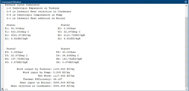
• fprintf :- This command used to display information in command window as output.
• \n :- To put enter in line
• %s :- To write string
• %f :- To write float values

  % Diplaying result
  
  fprintf('Rankine Cycle Simulator');
  fprintf('\n 1-2 Isentropic Expansion in Turbine');
  fprintf('\n 2-3 is Isobaric Heat rejection in Condenser');
  fprintf('\n 3-4 is Isentropic Compression in Pump');
  fprintf('\n 4-1 is Isobaric Heat addition in Boiler');
  
  fprintf('\n\n %1s %35s\n','State1','State2');
  fprintf('%s %5.3f%s %24s %.3f%s \n','P1:',p1,'bar','P2:',p2,'bar');
  fprintf('%s %.3f%s %21s %.3f%s \n','T1:',t1,'Deg C','T2:',t2,'Deg C');
  fprintf('%s %8.3f%s %20s %.3f%s \n','H1:',h1,'KJ/kg','H2:',h2,'KJ/kgK');
  fprintf('%s %.3f%s %22s %.3f%s \n','S1:',s1,'KJ/kgK','S2:',s2,'KJ/kgK');
  
  fprintf('\n\n %1s %35s\n','State3','State4');
  fprintf('%s %5.3f%s %24s %.3f%s \n','P3:',p3,'bar','P4:',p4,'bar');
  fprintf('%s %.3f%s %21s %.3f%s \n','T3:',t3,'Deg C','T4:',t4,'Deg C');
  fprintf('%s %7.3f%s %20s %.3f%s \n','H3:',h3,'KJ/kg','H4:',h4,'KJ/kgK');
  fprintf('%s %.3f%s %21s %.3f%s \n','S3:',s3,'KJ/kgK','S4:',s4,'KJ/kgK');
  
  fprintf('\n %30s %.3f %s','Work output by Turbine:',W_T,'KJ/kg');
  fprintf('\n %30s %.3f %s','Work input by Pump:',W_P,'KJ/kg');
  fprintf('\n %30s %.3f %s','Net Work:',W_net,'KJ/kg');
  fprintf('\n %30s %.3f','Thermal Efficiency:',Efficiency);
  fprintf('\n %30s %.3f %s','Heat input in Boiler:',Q_In,'KJ/kg');
  fprintf('\n %30s %.3f %s \n','Heat rejected in Condenser:',Q_In,'KJ/kg');
  ​

Plots :-

Output Screen :-