Project 1
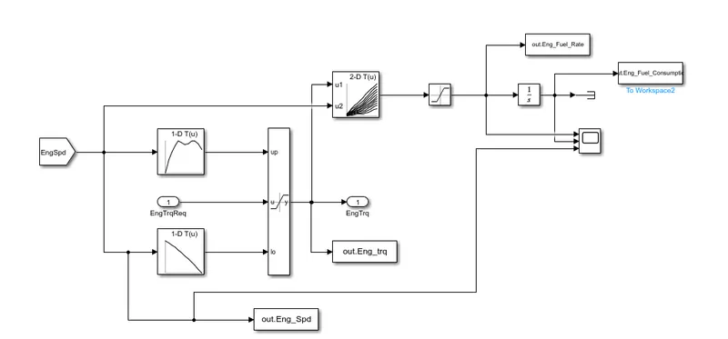
The engine and vehicle dynamics block :-
Engine Block :-
Vehicle Dynamics :-
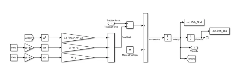
These above two blocks added in Simulink model.
Program of Plots for UDDS Cycle:-
%% Vehicle Parameters
M = 1500;       % Vehicle weight [kg]
Cr = 0.015;     % Rolling resistance coefficient
Rw = 0.35;      % Rolling radius [m]
Cd = 0.33;      % Drag coefficient
Af = 2;         % Frontal area [m2]
rhoa = 1.225;   % Air density [kg/m3]
Vwind = 0;      % Wind velocity [kmph]
g = 9.81;       % Gravitational acceleration [m/s2]
theta = 0;      % Slope [deg]
myu_road_tire = 1; % Coefficient of friction between tire - road interface

%% Powertrain Parameters
FDR = 3.73;                         % Final Drive Ratio / Diff Ratio
DiffEff = 0.99;                     % Differential efficiency (assumed independent of operating conditions)

NumGear = 4;                        % Number of gears in transmission
TransGear = [1:NumGear];            % Transmission Gears
TransRatio = [3.06, 1.62, 1, 0.7];  % Corresponding Transmission ratios
TransEff = 0.90;                    % Transmission efficiency (assumed independent of operating conditions)

TC_SR = [0, .5, .6, .7, .8, .87, .92, .94, .96, .97, 1];   % Torque Converter Speed Ratio (Matlab default) -> TurbSpd/PumpSpd
TC_TR = [2.232, 1.5462, 1.4058, 1.2746, 1.1528, 1.0732, 1.0192, 1, 1, 1, 1];   % Torque Converter Torque Ratio (Matlab default) -> TurbTrq/PumpTrq
TC_Cf = 1e-4 * [.72558, .66322, .63463, .59042, .51331, .4144, .29287, .22444, .12186, .04386, 0]; % Torque Converter Capacity Factor (Matlab default) -> PumpTrq/PumpSpd^2 [Nm/rpm^2]

load Vehicle_Data/Engine_data_1_9L_Saturn_95kW
load Vehicle_Data/Trans_Shift_map

%% Driver Parameters
Kp = 10;                    % P gain for driver PI model
Ki = 1;                     % I gain for driver PI model
Drive_Cycle_Select =1;     % Drive cycle selection

% Drive cycle values in m/s

if Drive_Cycle_Select == 1
    load DriveCycles/UDDS;

elseif Drive_Cycle_Select == 2
    load DriveCycles/HWFET;

elseif Drive_Cycle_Select == 3
    load DriveCycles/FTP;

elseif Drive_Cycle_Select == 4
    load DriveCycles/US06;

elseif Drive_Cycle_Select == 5
    load DriveCycles/NEDC;

elseif Drive_Cycle_Select == 6
    load DriveCycles/WLTP;

end

time_end = cyc_time(end);
vel_end = cyc_vel(end);

% Variables Define

t = out.tout;
TIS = out.Trans_In_Spd;
ES = out.Eng_Spd;
TOS = out.Trans_Out_Spd;
WS = out.Wh_Spd;

% Plot the time trace for engine, transmission input, transmission output and wheel speed

figure(1)

hold on
subplot(2,2,1)
plot(t,ES)
xlabel('Time')
ylabel('Engine Output Speed')

subplot(2,2,2)
plot(t,TIS)
xlabel('Time')
ylabel('Transmision Input Speed')

subplot(2,2,3)
plot(t,TOS)
xlabel('Time')
ylabel('Transmision Output Speed')

subplot(2,2,4)
plot(t,WS)
xlabel('Time')
ylabel('Wheel Speed')

hold off


% Plot engine torque, engine power, fuel rate and fuel consumption using subplots.

Eng_trq = out.Eng_trq;
Eng_pow = ES * pi / 30 .* Eng_trq / 1000;
Eng_fuel_rate = out.Eng_Fuel_Rate;
Eng_fuel_cons = out.Eng_Fuel_Consumption;

figure(2)

hold on
subplot(2,2,1)
plot(t,Eng_trq)
xlabel('Time')
ylabel('Engine Torque')

subplot(2,2,2)
plot(t,Eng_pow)
xlabel('Time')
ylabel('Engine Power')

subplot(2,2,3)
plot(t,Eng_fuel_rate)
xlabel('Time')
ylabel('Engine Fuel Rate')

subplot(2,2,4)
plot(t,Eng_fuel_cons)
xlabel('Time')
ylabel('Engine Fuel Consumption')

hold off


% Plot accelerator and brake pedal, gear command, vehicle desired and actual speed, vehicle distance using subplots

Acc_pdl = out.Acc_Pdl;
Brk_pdl = out.Brk_Pdl;
Gear_cmd = out.Gear_Cmd;
Vh_de_spd = out.Vehicle_Desired_Speed;
Vh_act_spd = out.Veh_Spd;
Vh_dis = out.Veh_Dis;

figure(3)

subplot(2,2,1)
plot(t,Acc_pdl)
hold on
plot(t,Brk_pdl)
xlabel('Iime')
ylabel('Paddle')
legend('Acc','Brake')
hold off

subplot(2,2,2)
plot(t,Gear_cmd)
xlabel('Time')
ylabel('Gear Command')

subplot(2,2,3)
plot(t,Vh_de_spd)
hold on
plot(t,Vh_act_spd)
xlabel('Time')
ylabel('Speed')
legend('Desired','Actual')

subplot(2,2,4)
plot(t,Vh_dis)
xlabel('Time')
ylabel('Vehicle Distance')

% Eng_map_trq

figure(4)

[a b] = contour(Eng_map_trq,Eng_map_spd*30/pi,Eng_fuel_map);
clabel(a,b)
xlabel('Engine Torque')
ylabel('Engine Speed')
title('Engine Fuel Consumption Map')

% Tabulate the fuel economy numbers (kmpl)

petrol_density = 0.7197;
kmpl = Vh_dis(end) / (Eng_fuel_cons(end) / 1000 / petrol_density)
1. Plot the time trace for engine, transmission input, transmission output and wheel speed
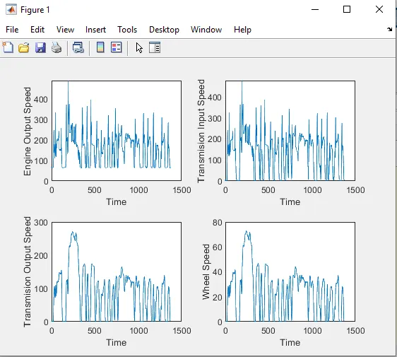
- Engine speed is fluctuating according to UDDS cycle load rquirement. But engine is not being off due to that engine RPM is being constant below 100 while in no load condition.
- Engine is connected with transmiion through clutch. While no load condition clutch disengage transmission with engine. So transmission input is being zero while engine idling as show in plot.
- Transmision speed is reduce due to friction and other minimal loss. Thats why output values are less than input values.
- This transmission output speed transfer to the wheel.And vehicle is start roling. Wheel speed is increase or decreased according to transmission output speed.
2. Plot engine torque, engine power, fuel rate and fuel consumption
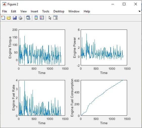
- As usual engine torque is increased as vehicle accelerate. Also torque value is going negative when vehicle is deaccelerate.
- This same pattern is followed by engine power. We can regen this negative torque or power to electiricity for using other places.
- Obviously, engine fuel rate is increase and decrease as vehicle speed increase or decrease.
- Fuel consumption is start as UDDS cycle start and increasing till vehicle will being off.
3. Plot accelerator and brake pedal, gear command, vehicle desired and actual speed, vehicle distance
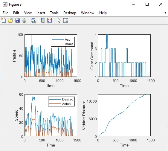
- First plot shows pedal position. As driver require more speed according to UDDS cycle it press more acceleration pedal. And while deacceleration it press brake pedal according to deacceleration requirement.
- As speed increase and decrease drive change gear shifter according to speed requirement. Higher the speed higher the gear ratio.
- In third plot, actual vehicle speed is less than desired speed due to friction and operation feedback delay and many other fatigues.
- Vehicle is start moving while UDDS cycle introduce to vehicle and keep increasing till vehicle stops or engine is getting off.
4. Plot the engine operating points
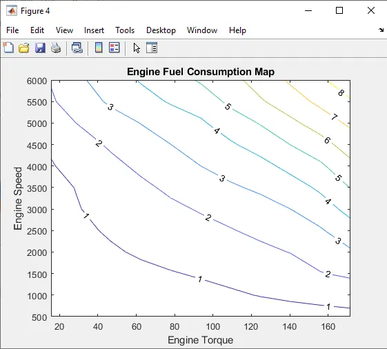
- In fuel consumption contour map, it is conclude that fuel consumption is same as Lower speed and higher torque as higher engine speed and lower engine torque.
5. Fuel economy numbers (kmpl)
kmpl = 1.4204e+04
Plots for HWFET Cycle:-
1. Plot the time trace for engine, transmission input, transmission output and wheel speed
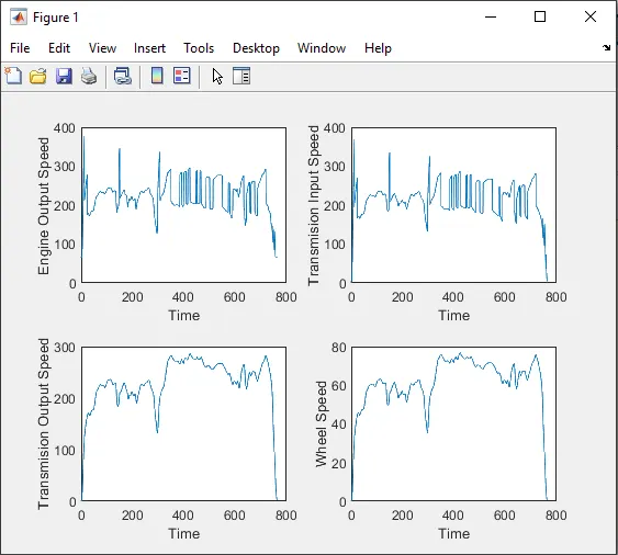
- Engine, Transmission and Wheel shows same observaion as UDDS cycle only variation in speed is decreased.
2. Plot engine torque, engine power, fuel rate and fuel consumption
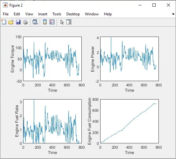
- Every comments on this plot is same as UDDS cycle. Only working range of plot is converge due to less speed fluctuation.
3. Plot accelerator and brake pedal, gear command, vehicle desired and actual speed, vehicle distance
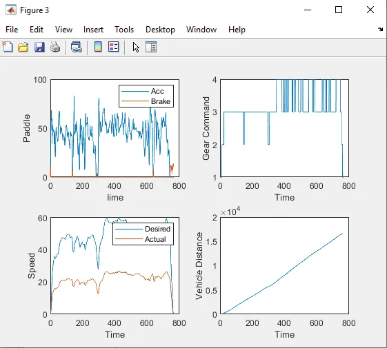
- Plot obsevations are same as UDDS cycle. Only vehicle is mostly running on 3 or 4th gear due to less speed fluctuation.
4. Plot the engine operating points
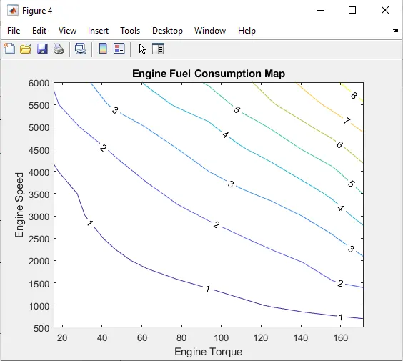
- This plot is as same as UDDS plot. There is no change in plot.
5. Fuel economy numbers (kmpl)
kmpl = 1.6501e+04
- Fuel economy number is more for HWFET than UDDS due to higher fuel rate to maintain high speed constantly.