Plotting a Function using Simulink

1. AIM

1. Plot a function `y(x) = (x-1)*(x-3)^2*(x-9)^2` using basic simulink blocks.
2. Run the Simulink example 'Suspension System Comparison'.

2. OBJECTIVE

• To understand the basics of Simulink, the library browser, and the different blocks which are used in Simulink.
• To run the example file and compare the results.

3. METHOD

3.1 Block Diagrams for the plot of y(x)

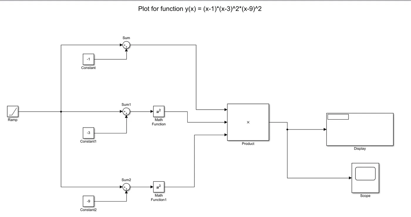
For plotting the y(x) function we can use two methods. We can use a ramp block as our input block or we can use 'x' as our input.

• Using Ramp block

BLOCK DIAGRAM IN SIMULINK USING RAMP BLOCK

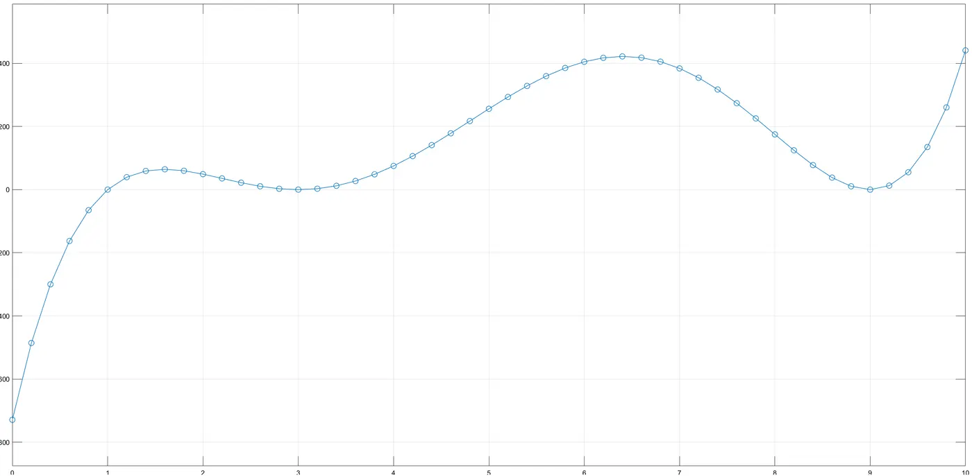
• When using the Ramp block the value of 'x' will increase for every second. We run this simulation for 10 secs and we get the plot for this.
• Here the Ramp block will act as a loop and iterate the values of x.
• We get the plot for the above simulation as

PLOT FOR RAMP BLOCK

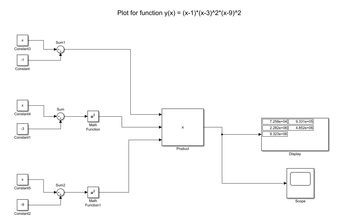
• Using constant block with x as input

BLOCK DIAGRAM WITH CONSTANT BLOCK

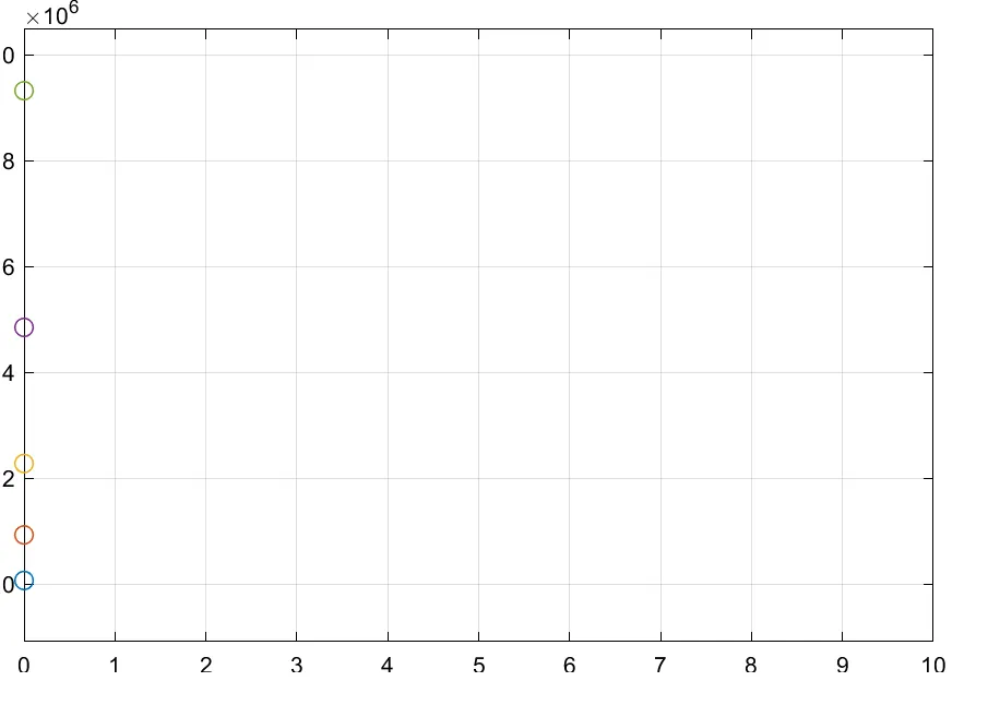
• Here 'x' values can be given as input variables. The values can be input from the command window.
• We get the plot as

PLOT FOR CONSTANT BLOCK

3.2 Basic blocks used for the block diagrams above

	The Ramp block generates a signal that starts at a specified time and value and changes by a specified rate.
	The Constant block generates a real or complex constant value signal.
	The Sum block performs addition or subtraction on its inputs.
	The Math Function block performs numerous common mathematical functions.
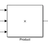	The Product block outputs the result of multiplying two inputs: two scalars, a scalar and a nonscalar, or two nonscalars that have the same dimensions.
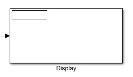	The Display block shows the value of the input data.
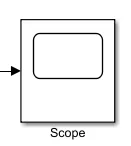	The Simulink Scope block display a time-domain signal.

3.3 Answers for the questions asked

Objectives of simulation

• Simulation is the virtual environment which is fictitious setups of systems. The model is run through the simulation to depict real-world behavior as the main focus for the outputs.
• To make actual systems its time consuming and costly, so the simulations for such experiments are better since they are fast and we can avoid financial risk.
• The main plus point of doing simulations is that we can speed up the flow of time. We can get results quickly in simulations which may take up a long time if performed in real life.
• All the logical operations and equations can be converted into blocks. So we can make a simplified version of a complex system in form of block diagram.
• Simulations can be used for the following things

1. Performance analysis - How well the system performs under certain conditions in all measures of significances.
2. Capability analysis - We can determine if the system has the ability to meet up with the performance requirements and criteria.
3. Comparison study - We can compare different configurations or design variations of the system with one another.

Similarities and Differences between the three systems understudy

1. First shock absorber - It uses a shock absorber block with linear stiffness and damping.
2. Second shock absorber - Uses Nonlinear Transitional Spring and Nonlinear Transitional Damper specified by symmetric polynomials.
3. Third shock absorber - Uses Variable Transitional Spring and Variable Transitional Damper.

The spring constant is varied during the simulation using open-loop control and the damping coefficient adjusts to ensure critical damping is achieved. Closed-loop control can be added to simulate an adaptive suspension system.

The example 'Suspension System Comparison' shows these above-mentioned spring and damper systems excited by the same oscillating velocity source.

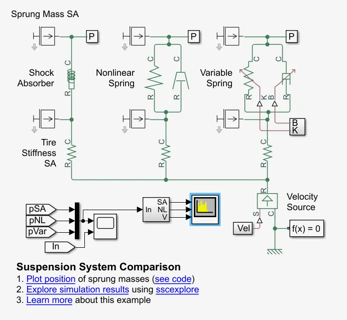SUSPENSION SYSTEM COMPARISON BLOCK

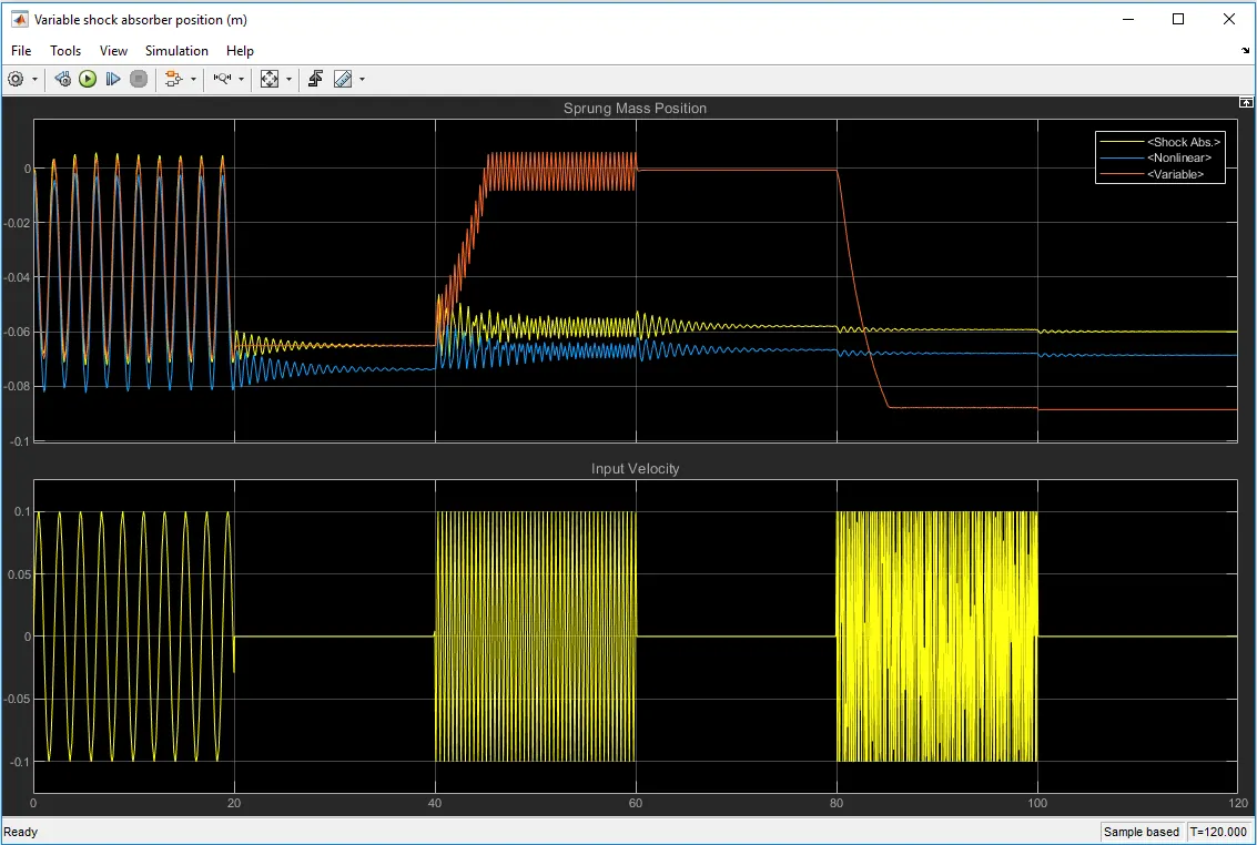fig. showing the sprung mass position

Observations from the results

• The plot above shows the position of sprung masses in the three different suspension models that are subjected to the same test.
• From the plot, it is seen that the first pulse generated by the sine wave is a little wider having frequency 3 and phase delay of 0, as the frequency and phase delay increases the output increases.
• This variation exists between 0-20, 40-60, 80-100.

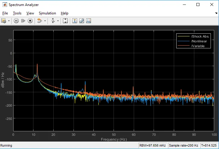fig. showing the power spectral density analysis

Oscillating Velocity Source

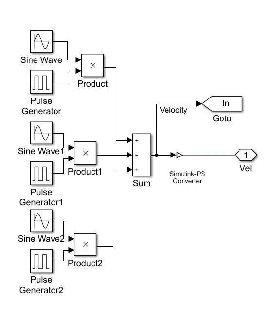OSCILLATING VELOCITY SOURCE

• The velocity source used in the above comparison is the oscillating velocity source.
• The velocity is constantly changing, oscillating same as the displacement.
• Three sine wave blocks and 3 pulse generator blocks are used to create the source.

4. LEARNING OBJECTIVE

1. To learn the basics of Simulink.
2. To understand how to simulate models in Simulink to plot a function.
3. To understand how the example models in Simulink are run and compare the results of the outcomes.

5. CONCLUSION

We can use 'x' as a constant block and assign some variables to 'x' and get the output for the plot.

We can also use the Ramp block as the input as it also acts as a loop which is like a for loop.

Output plots for both are shown as results.