MATLAB - Genetic Algorithm
1. AIM
To write a program in MATLAB to optimize the stalagmite function and find the global maxima of that function.
2. OBJECTIVE
- To make a stalagmite function to find the global maxima(maximum peak value).
- To make a program to optimize the above function.
- To understand the concept of genetic algorithm (ga).
3. METHOD
3.1 THEORY
Optimization
- When it comes to engineering systems like IC engines, wings of the aircraft, etc. there are many particular things that it has to do properly.
- when it comes to airfoils it needs to provide proper lift at different angles of attack and it should also reduce drag. So for different conditions, the drag value should be minimum.
- So to modify the best design combination to reduce drag we cannot use a brute force method like checking each and every combination as it will take a lot of time. So to find the best combination optimization is used.
- Optimization in an area of study which deals with how to minimize or maximize a function which depends on multiple input parameters.
Stalagmite Function
- It is a mathematical model that helps us generate local maxima or minima.
- It is a 3-D function.
- It is made up of many local maxima and the big peak is the global maxima.
- The objective of an optimization study is to determine the global maxima or minima without having any prior knowledge of this particular field.
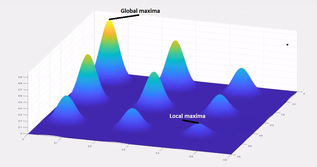 |
| Fig1. Plot showing the local and global maxima of the stalagmite function |
Genetic Algorithm
- The genetic algorithm is based upon the 'Theory of Evolution' which was proposed by Charles Darwin.
- It is based on random sampling, in which we start with random inputs, and based on those inputs we evaluate the function, then we apply the concept of natural selection where we take 2 generations and basically mutate them and do cross over and then we create a new generation that is hopefully better than the last.
- It is an inbuilt function in MATLAB.
- Note: by default, it always minimizes the function.
x = ra(fun,nvars)- finds a local unconstrained minimum, x, to the objective function, fun.
- nvars is the dimension (number of design variables) of fun.
Outline of the ga algorithm
-
The following outline shows how the genetic algorithm works:
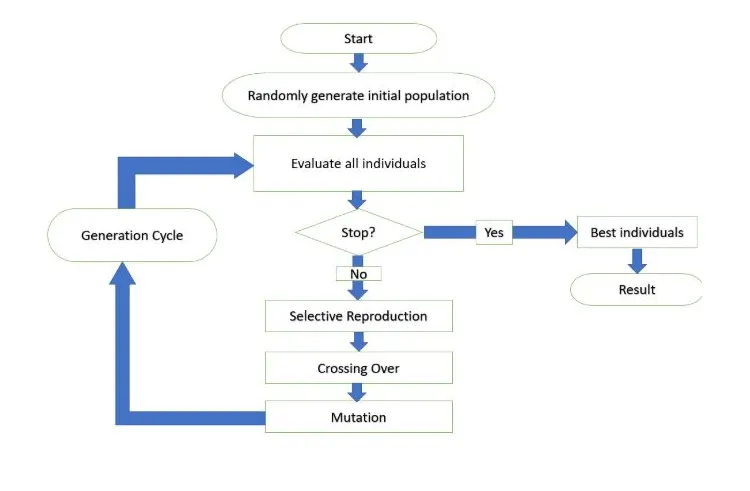
- The algorithm begins by creating a random initial population.
- The algorithm then creates a sequence of new populations. At each step, the algorithm uses the individuals in the current generation to create the next population.
- To create the new population, the algorithm performs the following steps:
- Scores each member of the current population by computing its fitness value. These values are called the raw fitness scores.
- Scales the raw fitness scores to convert them into a more usable range of values. These scaled values are called expectation values.
- Selects members, called parents, based on their expectation.
- Some of the individuals in the current population that have lower fitness are chosen as elite. These elite individuals are passed to the next population.
- Produces children from the parents. Children are produced either by making random changes to a single parent—mutation—or by combining the vector entries of a pair of parents—crossover.
- Replaces the current population with the children to form the next generation.
- The algorithm stops when one of the stopping criteria is met.
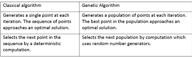 |
| Difference between classic and genetic algorithms |
 |
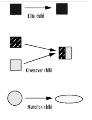 |
| Flow chart of how the ga algorithm works | figure: how children are produced |
3.2 MATLAB Program
% Program of optimize Stalagmite function and find the global maxima

clear all
close all
clc

% Input of 1-D arrays
x = linspace(0,0.6,150);
y = linspace(0,0.6,150);
num_cases = 50;

% Creating 2D mesh
[XX YY] = meshgrid(x,y);

% Evaluating the stalagmite function
for i = 1:length(XX)
    for j = 1:length(YY)
        input_vector(1)=XX(i,j);
        input_vector(2)=YY(i,j);
        f(i,j) = stalagmite(input_vector);
    end
end

tic % to measure time taken
% Study 1 - Statistical behavior with no constraints
for i = 1:num_cases
    [inputs, fopt(i)] = ga(@stalagmite, 2);
    xopt(i) = inputs(1);
    yopt(i) = inputs(2);
end
study_time1 = toc

% Plotting graph for Study 1
figure(1)
subplot(2,1,1)
hold on
surfc(XX,YY,-f)
shading interp
plot3(xopt,yopt,-fopt,'marker','o','markersize',5)
title('Inputs')
subplot(2,1,2)
plot(-fopt)
xlabel('No. of Iterations')
ylabel('Function Maximum')

tic
% Study 2 - Statistical behavior with Upper and Lower bounds (0 and 0.3)
for i = 1:num_cases
    [inputs, fopt(i)] = ga(@stalagmite, 2,[],[],[],[],[0;0],[0.3;0.3]);
    xopt(i) = inputs(1);
    yopt(i) = inputs(2);
end
study_time2 = toc

% Plotting graph for Study 2
figure(2)
subplot(2,1,1)
hold on
surfc(XX,YY,-f)
shading interp
plot3(xopt,yopt,-fopt,'marker','o','markersize',5)
title('Inputs')
subplot(2,1,2)
plot(-fopt)
xlabel('No. of Iterations')
ylabel('Function Maximum')

tic
% Study 3 - Stastical behaviour after increasing the population size
options = optimoptions('ga');
options = optimoptions(options,'PopulationSize',180);

for i = 1:num_cases
    [inputs, fopt(i)] = ga(@stalagmite, 2,[],[],[],[],[0;0],[0.3;0.3],[],[],options);
    xopt(i) = inputs(1);
    yopt(i) = inputs(2);
end
study_time3 = toc

% Plotting graph for Study 3
figure(3)
subplot(2,1,1)
hold on
surfc(XX,YY,-f)
shading interp
plot3(xopt,yopt,-fopt,'marker','o','markersize',5)
title('Inputs')
subplot(2,1,2)
plot(-fopt)
xlabel('No. of Iterations')
ylabel('Function Maximum')
Idea behind the code
- Start with clear all, close all, clc.
- Create a 1-D array, x and y.
- Using above 1-D array make a 2-D mesh using meshgrid(x,y).
- We use num_cases to run for 50 iterations.
- Then we evaluate the stalagmite function using double for loop.
- Then we make 3 studies, and we refine the optimization process with each study until we find a single maxima
- We use subplot for making different plots in the same figure window.
- plot(X, Y, -f) the ga calculates optimum values for 50 iterations for every possible input.
- To measure how long it takes for each study to run we use the tic - toc command.
- surfc() is used to plot a 3-D graph.
- shading interp command is used for shading the graph instead of plotting lines on the graph which provides a smoother graph.
3.2.1 Study 1
- we have not provided any boundaries and there are no constraints for study 1 so the code will give different outputs each time the code runs resulting in the following plot.
- Here when we plot the stalagmite functions, the values of ga are all over the place due to random sampling.
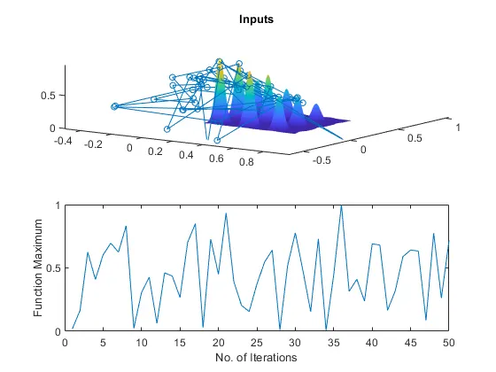 |
| Fig2. Plot for Study 1 |
3.2.2 Study 2
- In this study to solve the above issue we need to bound the upper and lower values and it is done using the following syntax.
x = ga(fun,nvars,A,b,Aeq,beq)- This finds a local minimum x for func, subject to the linear inequalities Aeq*x = beq and A*x>= b
- Set A=[] nad b=[] if no inequality exists.
- So the bounded plot is shown below.
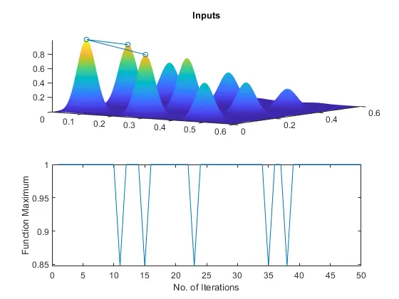 |
| Fig3. Plot for Study 2 |
3.2.3 Study 3
- In addition to the bounds we also change the initial population size to 180.
- Since the ga algorithm uses brandon sampling, the initial population size is set to 50 by default.
- It helps in the plotting of the local and global maxima a bit better since we have a large population size instead of 50.
- The only drawback is that it slows it down.
- we use the options part of the ga to make changes to the population size.
- hence we get a single peak.
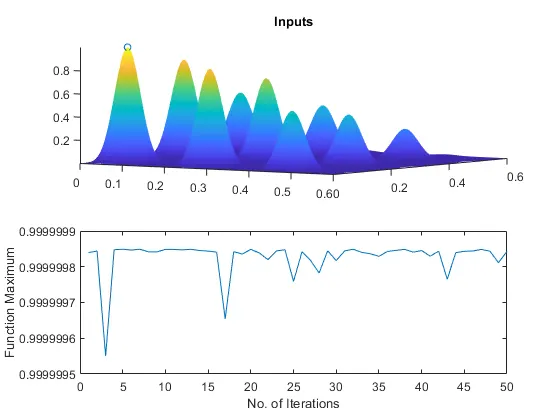 |
| Fig4. Plot for Study 3 |
3.3 Stalagmite Function
% Stalagmite function for maximization

function [f] = stalagmite(input_vector)

XX = input_vector(1);
YY = input_vector(2);

f1x = (sin(5.1*pi*XX+0.5))^6;
f1y = (sin(5.1*pi*YY+0.5))^6;

f2x = exp(-4*log(2)*((XX-0.0667)^2/0.64));
f2y = exp(-4*log(2)*((YY-0.0667)^2/0.64));

F0 = (f1x*f1y*f2x*f2y);

f = -F0; % '-' the minus sign is used for maximization

end- The code gives an idea of what the stalagmite function is.
- The code is a function generated for the program.
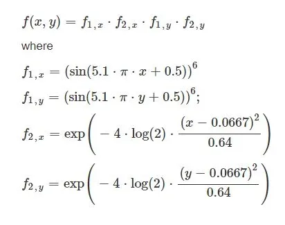
- The formula is for finding minima and we use the minus sign for modifying the formula to find maxima.
- The formula for the above code is given below.
3.4 Stopping Criteria for the GA algorithm
These are the conditions used by genetic algorithm to determine when to stop
- MaxGenerations - it stops when the number of generations reaches MaxGenerations.
- Maxtime - it stops after running for an amount of time in seconds which is equal to MaxTime.
- FitnessLimit - it stops when the value of fitness function for the best point in the current population is less than or equal to FitnessLimit.
- MaxStallGenerations - it stops when the average relative change in the fitness function value over MaxStallGenerations is less than FunctionTolerance.
- MaxStallTime - it stops if there is no improvement in the objective function during an interval of time in seconds equal to MaxStallTime.
- FunctionTolerance - it runs until the average relative change in the fitness function value over MaxStallGenerations is less than FunctionTolerance.
- ConstraintTolerance - The ConstraintTolerance is not used as stopping criterion. It is used to determine the feasibility with respect to nonlinear constraints. Also, max(sqrt(eps),ConstraintTolerance) determines feasibility with respect to linear constraints.
3.5 Significance of running multiple iterations
- we run multiple iterations so that we get a more accurate result.
- when we increase the number of iterations we can refine the result.
4. LEARNING OUTCOME
- Learned the use of a stalagmite function.
- Learned how the ga algorithm works.
- Learned how to change the various values in ga so that we get a more accurate reading.
5. CONCLUSION
The Global maxima is calculated using the ga algorithm but the stalagmite function needs to be inversed so that we can get the global maxima instead of global minima.
6. REFERENCES